Installing Tensor Flow for GPU

The TensorFlow website provides a brief outline of how to get a tensorflow programs running on an NVidia card but due to updates on the NVidia site, some of the instructions are a little hard to follow and it is easy to make a mistake, so I will give an updated guide here.

STEPS

• Run DDU, a tool for removing current display drivers from your computer.
  DDU removes the current NVidia driver from your computer and any associated files. This prevents the a common error when rolling back to older NVidia drivers. 
• Install the CUDA Toolkit version 9.0. This toolkit comes with the correct driver version for using it. There are newer versions of the toolkit now, but version 9.0 is what is required for TensorFlow-GPU. If the link here breaks, this version of the toolkit is found in the archives.
• Install cuDNN v7.0.5 (Dec 5, 2017), for CUDA 9.0. Like the CUDA Toolkit there are newer versions of this tool, so this one is found in the archives. 

The TensorFlow website suggests to set the correct PATH variables in Windows according to the documentation - but in my experience with these specific installers that is done during the installation process.

Once everything is installed and you have restarted your computer you can install tensorflow-gpu from pip or through Anaconda

pip3 install --upgrade tensorflow-gpu

Then you can run the test python scripts found here to validate the GPU support. 
NOTE: There is a rather nasty bug in the example GPU scripts - when it suggests to test a maximum percentage usage of memory on the GPU ensure that the maximum number you set is less than what is currently available. Any contention for memory on the GPU causes a hard driver crash.

With that all up and running - enjoy much faster machine learning!

What can we learn from GPU Frame Captures: Stardew Valley

If you read my last post on frame captures we discussed how GPU frame captures can be used to analyse performance, and determine how a scene is rendered for a specific game. 

It also gives insight into what the game is doing right (from a performance perspective) and how it can be improved.

In the last post we looked into Europa Universalis 4 where we found an astronomical amount of draw-calls, strange scaling behaviour and sub-optimal texture packing to render a relatively simple (although quite large) world.

In this post we are looking at a retro game for comparison. Many people who havent kept up with modern graphics development may believe that modern "retro" looking games use the same old rendering techniques that used to be mandatory on the old consoles - this isn't the case!

Stardew valley mimics the aesthetic of old SNES games like Harvest Moon but the process by which it draws the scene makes it more dynamic, smooth and pretty doing many things that would have been impossible back then to make a great experience now.

Rendering Pattern

The rendering pattern is very simple for this 2D game. It follows the expected patternn of drawing the floor and background followed by a distance sorted order of objects. In a 2D game with this view, the objects "further away" are those higher-up the screen as they will not obscure those further down. This allows the renderer to not have to worry about depth testing.

The full pattern for rendering as I could figure it out from a capture appears to be:

In this pipeline the only steps which really take any time are the two full screen passes, they are the initial ground rendering after the screen clear, and the full-screen weather effects- in our case, snow.

The initial ground rendering is a simple tiled geometry representing the game world grid and each grid cell has UV coordinates to map to a cell in the bound ground textures. 

The snow rendering is similar but mapping to a different section of the texture as shown below:

The snow is then animated by updating which cell is read for each game-world quad each frame. Notice that the background for the snow texture is not black, it is a dark grey. This is what adds the hazy effect to the scene as the texture is not directly written to the scene as the other blocks have been, it is an additive effect (D3DBLENDOP_ADD) resulting in softening of the image.

All in all it produces a quite nice, and retro effect - even though this approach might be too intensive for most real "retro" games.

Another interesting feature of this game is that it lets you customise how your character looks. Instead of using those options to generate a new sprite sheet for rendering your character, the game instead keeps all the possible options in memory and builds up the character chunk by chunk based on your choice from these options, each frame.

This is a neat and simple trick that avoids having to create a new texture when a game is loaded - but limits the extension and number of choices for the player as adding any new options increases the memory usage of the game through the entire run-time, although this is probably trivial on a game of this scale.

So how do we improve on this?

A game of this scale and already tiny frame rendering times (<2ms) there isnt really any need to improve anything. Unless you were running an incredibly outdated machine this game will run incredibly well.

However, if we were thinking of running this game on a very limited device we would probably want to consider the techniques that were used on the actual old retro games.

For starters, the majority of the scene (with an exception of the weather effects) doesn't change frame to frame - and those bits which do are somewhat predictable. There is no reason why parts of the scene couldnt be rewritten as things or the camera move and otherwise kept the same - this would infact throw out a majority of the draw-calls when the camera is stationary. The draw backs to this approach is that any mistakes in the implementation have really ugly artefacts.

This game also falls prey to the same issues as EU4 when it comes to texture sizes (although most are trivial in this case making the slight error not too big of a problem).  There are a number of large textures in this game that are just slightly above a power of two texture size - resulting in some wasted memory.

Otherwise, this frame capture is incredibly nice and easy to investigate and navigate.

What can we learn from GPU Frame Captures: Europa Universalis 4

A common technique used in the games industry to analyse the state of a game in development and look for where improvements can be made is to capture a frame(all the GPU work being done between each frame being shown to the user) from the game and analyse the results to see the impact of the different elements on the screen and how they might be able to be rearranged.

In doing this we can look at the relative costs of the different aspects of the processes in the scene. An example of this would be that the programmer suspects that the newly implemented bloom post-effect has had too big an impact on performance. So the programmer grabs a few frames from the game and looks at the time that is being taken to perform that effect at different places in the game, and what the cost of that is relative to the rest of the scene.

Another use for this approach is for new programmers coming onto a complex project to get a quick look at the rendering 'pipeline' that has been implemented. As in, what is rendered when, by what shader and in what order. This is quite useful for someone who only needs to make a minor change on a project.

An interesting side-effect of this is that we are able to frame-capture fully finished games and look at what the code is asking our computer to do and from that derive how the rendering system of that game works to some extent.

In this post we will be looking at Europa Universalis 4(EU4) frame captures and constructing a flow chart of how that game is rendered. EU4 is the forth game in the Europa series from Paradox Interactive released in 2013.

To capture frames from the game we will be using Intel's GPA. GPA is one of the simpler and less detailed frame capturing tools available but is good enough for this example and will allow someone with GPU to be able to follow along if they wish.

(For those interested in more complex capture tools the most popular amongst those I know in industry is RenderDoc, but AMD and NVidia each have there own tools which provide specific functionality for features of their cards in Radeon GPU Profiler and NVIDIA NSight respectively. Microsoft also have a tool called PIX but I haven't personally used that in some time but have heard it works with AMDs tools now.)

First thing we want to do is use the GPA Graphics Monitor tool to launch EU4 from its directory. This will launch the game with the GPA overlay, giving us real-time performance information and the option to capture frames. In this example I will be running on a NVIDIA 1080 GPU so will be targeting the max settings so that we can see where each option is placed in the pipeline. The settings and overlay can be seen in the screenshot below.

The intention was to run with max settings, but we have had to step down from 4k to 2560x1440 due to the game performance dropping to below 1FPS at the higher resolution while running with Intel GPA (and not good without it either...) . Something that will be covered later.

With the settings covered and GPA running we now need to take some frame captures. As this game has a relatively simple view, we will be taking a capture close to the ground, mid-zoom out and full zoom-out to get a full coverage of the some of the most common cases.

This is performed by pressing Ctrl+Shift+C when the game is in the right position. An important note when capturing is to take note of the CPU usage. This data is not always captured with the frame and can indicate if there is a CPU bottleneck which may be causing poor GPU performance. In the case of our capture (below) we arent using very much CPU at all so that should not impact the results much here.

In my captures I have used a save file from a playthrough with a random 'new world'. This is due to my own interest in seeing if the randomly generated terrain is handled differently than the standard world map geometry.

Once the three captures have been taken, open Intels Graphics Frame Analyser tool where the captures should be displayed.

We can start by opening the zoomed-out capture first, as this has the least detail and should give use the broad strokes of the rendering process. This will give you a view of the data like this:

The important things to look at here are the top timeline and the view frame at the bottom left. The timeline on the top will allow you to set the x and y axis to be the GPU duration to highlight particularly expensive calls and the view on the bottom will highlight what is being rendered on each render target for each of the calls in the timeline.

As an example I selected the group of similar draw calls (ID=~1000 to ~10400) which is appears to handle only the drawing of the borders in of the world and this is shown in the bottom frame with a pink highlight of the pixels which are being rendered to. Above that there is information on my selection. It says that we selected 9483 draw calls which account for 90.1%(!!!) of the total rendering time for the frame! Scary, but we will get to that in the section on how to improve this pipeline. For now this is just to show you how this tool works.

We will use this approach to see how the scene is rendered by stepping through the draw calls and seeing what they are doing. From what we can gather the process for drawing the world appears to be starting with the zoomed out capture:

Zoomed-out capture analysis
 

With the numbers referring to the GPU instruction ID

The timeline is broken up by some taller commands, there are the buffer copies which nicely split the pipeline into the four coloured sections shown in the diagram. The length of each section is not entirely representative of the total rendering time but is an indicator that something isn't as ideal as it could be in this particular pipeline.

Overall the pipeline is relatively simple (by modern standards). It uses a depth map for correctly layering objects in the scene and each stage of pipeline ties nicely into the options from the settings. With the exception of shadows which appear to be disabled or not rendering at this level of zoom. 

From a graphics programmers view, there is a number of very interestingly strange things going on with the way objects are submitted for drawing in this pipeline.

For starters the sheer number of draw calls is ridiculously large for even a major AAA game and this leads to a bottleneck in the gpu as each of the submitted draw calls are relatively tiny with only tens of primitives at the best of times. This is shown, rather crudely, in GPA by the occupancy and thread dispatch boxes showing red for the frame.

This is starving the GPU. For a lot of these calls the GPU is probably spending more time in the driver than it is actually processing the data it is being given. This is particularly noticed when the game is rendering borders, state names, rivers and trees.

The terrain is also interesting. The world is rendered as 36, 8196-triangle grids. Essentially one big height map broken into chunks, which reads its lighting from the precomputed base texture in the setup stage. 8196-triangles is a relatively insignificant amount of triangles to draw and each of the 36 grids appears to share the same texture and shader state. There doesn't appear to be an apparent reason this is separated instead of being one giant geometry. If the reason is LOD (level of detail) related this could be resolved CPU side very cheaply to select and combine multiple vertex buffers or vertex buffer sections into one call.

There is a lot of other details but they appear to be the same throughout all captures, so I will address them in the optimisation section at the end.

Close Capture Analysis

As suspected,. the shadows showed up in the close zoom levels. In the zoomed out pipeline map there was some strange depth maps being cleared and appeared not to be used later in the pipeline. When we have a closer view these render targets become used for storing and processing the shadow map that is produced in the setup stages, the shaders being used later in the pipeline are also binding this as a texture and appear to be using it - the rest of the pipeline remains unchanged in my casual exploration.

The borders, text and UI remain as the main culprit of GPU use, but with the additional of a lot of calls rendering the scene objects for the shadow map and processing adding some extra work.

This is offset by some good culling of the terrain. In the far out LOD the entire terrain and water were rendered as many chunks together. At this level, the fewer chunks reduces the total number of draw calls submitted, but the culling was not correct and some out of view chunks were submitted.

Mid-Zoom Capture

Our mid-level capture appears to have the same pattern as the far-out zoom. All the city, unit detail and shadow is LOD'ed out, leaving only the map rendering. The gives us the same behaviour with less of the draw-calls as less is visible. Rendering borders still covers the majority of the calls, but it isnt as dramatic as the far out zoom.

We can see in this image that the depth buffers used for the shadow map are still bound and cleared each frame (RT2-5) and are apparently unused, but I may have missed something.

Sins of a Render Empire

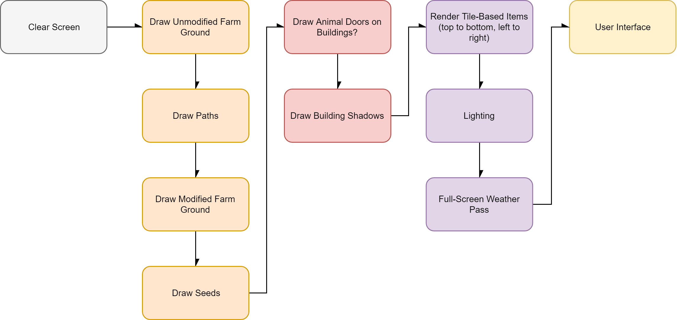
So in the last three sections I gave an overview of the pipeline and how it changes in different configurations - essentially some features are disabled as LOD features based on distance. However, this isnt the only place to look when we are considering performance. So in this section we are going to cover a few oddities that need addressing if this game was going to be optimised.

4k Support

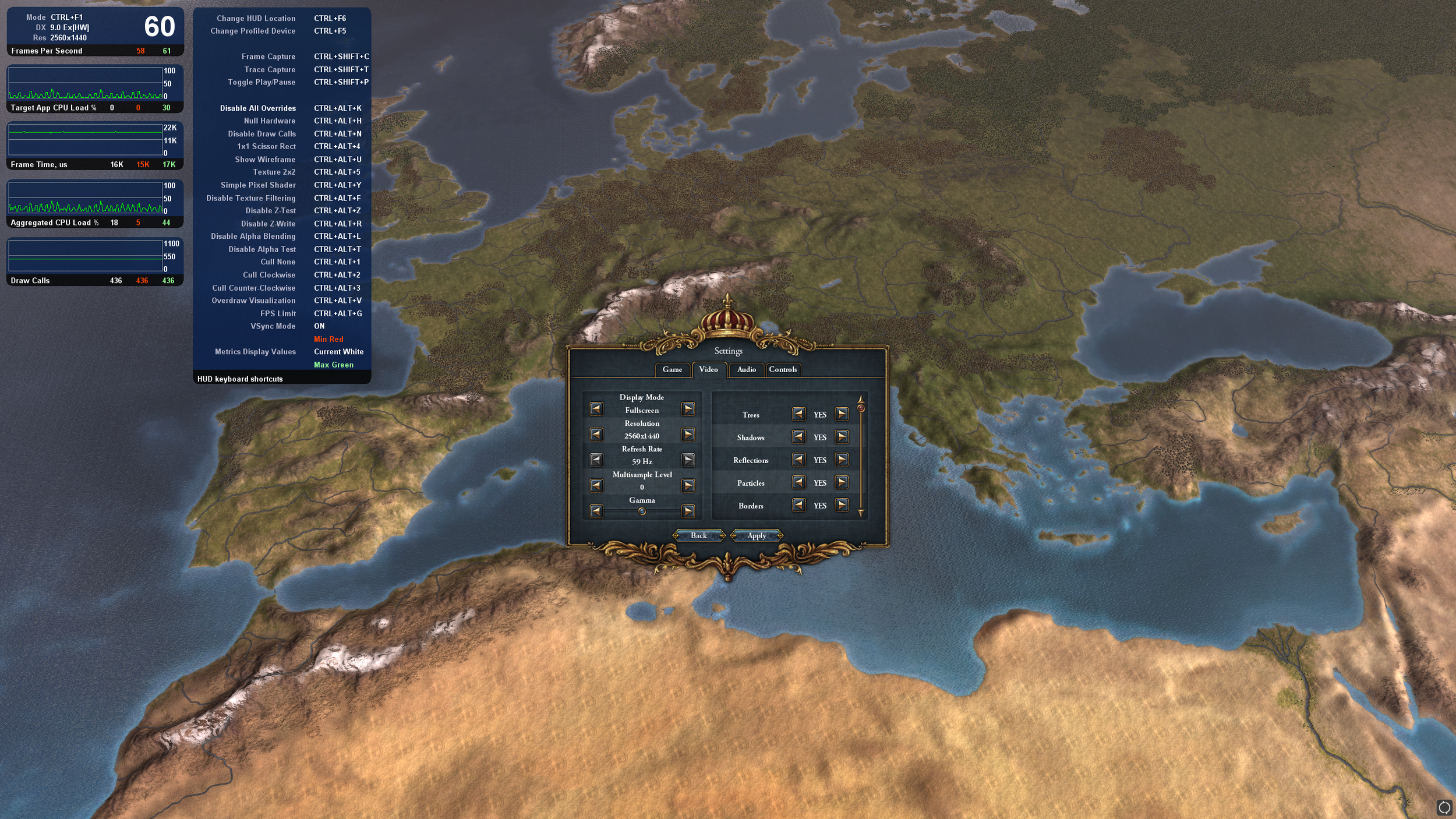
As I mentioned in the setup for this, I intended to run this on max setting at 4k resolution. This currently isn't possible with a high-end intel chip and NVidia 1080 - a little strange for a game from 2013.

The game runs roughly fine at 4k when we dont enable all the on-off options in the video menu. A quick investigation into this and it seemed that the shadows really take most the time. A problematic quirk of resolutions is that when we double the size we quadruple the number pixels (which also quadruples the amount of work). In this engine, the shadow buffers appear to be sized based on the full rendering resolution. So, going from 1440p to 4k doesnt just quadruple the cost of rendering the scene, it has to be rendered twice at that size, so it is a ~8x increase in rendering cost. 

Additionally the trees are expensive at 4k. This is a relatively simple reason, at 4k we see more pixels on each tree. Each tree has high texture detail and for some reason a detailed normal map. So now we have also quadrupled the texture read cost, with little coherency because the trees are small and dense and the texture resolution is reasonably high.

Water is similarly effected, but not as much as the trees due to similarity in the pixel space helping cache coherency.

In the game there are a number of what appear to be generated textures, the size of these appears to be loosely based on the resolution that is being used. However, they do not stick to power of two texture sizes. So a texture that is 1029x1029  is actually a 2048x2048 texture under the hood on certain hardware, this doesnt effect the appearance of the texture but does have performance implications and is just a massive waste of memory.

This next complaint is just because I play this game a lot. At 4k the menus get really tiny and that's a pain.

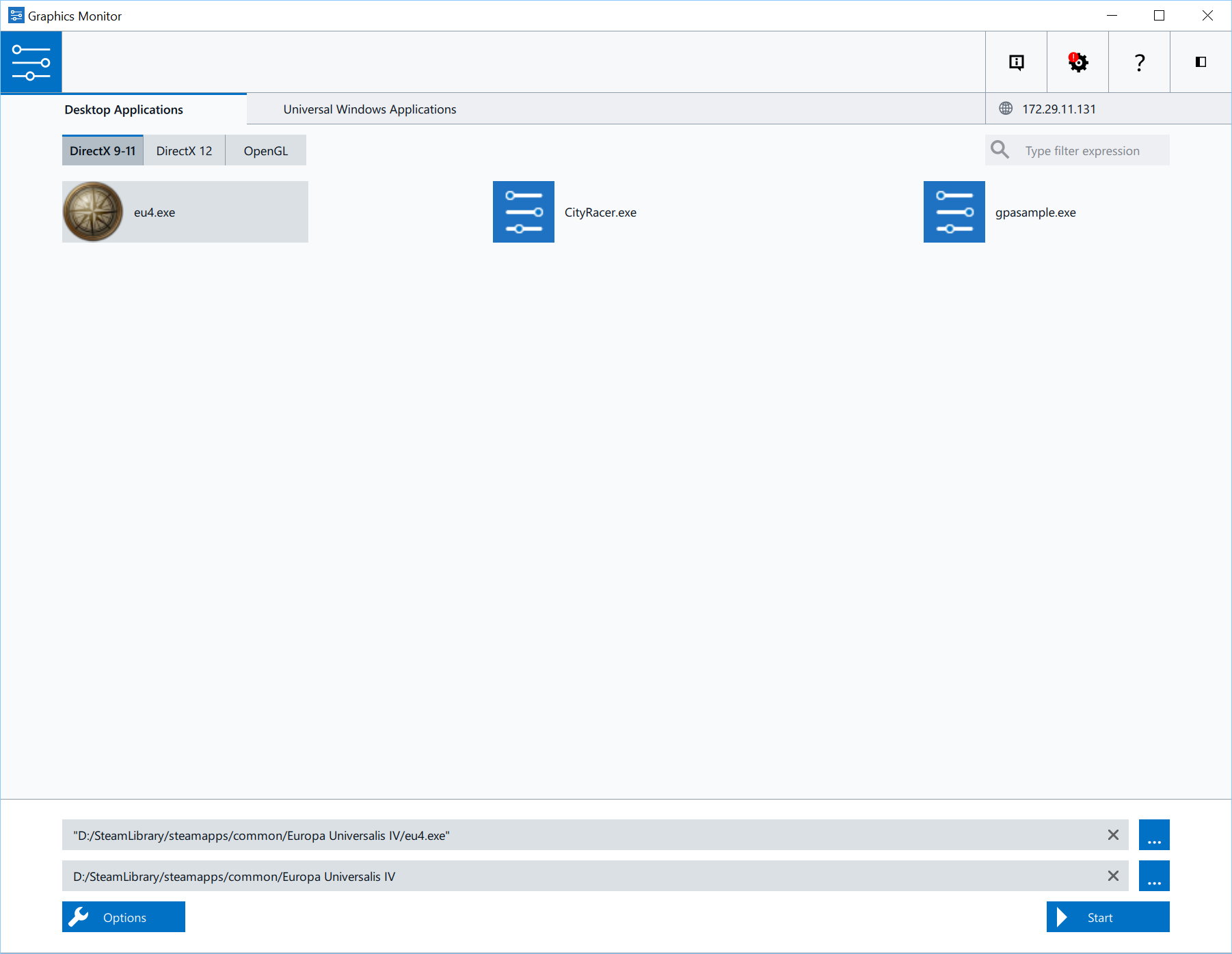
DirectX 9.0c

This game is written with DirectX 9.0c. In 2013 when this came out, DirectX 10 and 11 had long been a standard and DirectX 12 was well on the way as well as AMD's early experiments with Mantle which led to Vulkan.

AMD and NVIDIA put a lot of work into optimising drivers for modern hardware. This focus is obviously for patterns and use-cases in common software. DirectX 9.0c misses a lot of features that could really make this type of game fly on even a basic laptop.

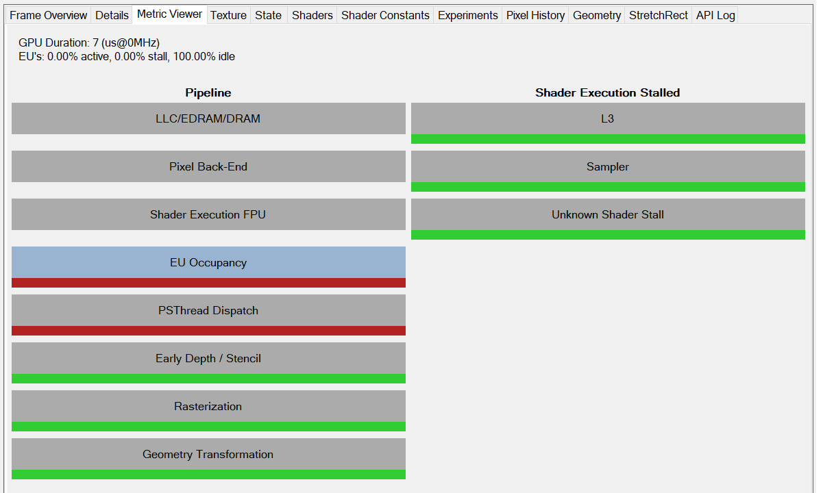
Overbinding and draw calls

Textures are bound each time they are used. Tiny objects are submitted to draw calls. There is either a massive lack of batching or it is not apparent in the capture.

This puts the game at the mercy of the PCI-bus and the drivers. Every time you ask the GPU to do something you risk a major state change stalling the next draw. So much of the textures being bound are identical (outside of the UI) and there is a lot of texture slots to bind, some textures are so low resolution they may as well be constant buffers and allow for some nice out of order operations to be able to be done.

Texture Space Wastage

The cubemap for the sea is a good example of this. Due to the angle of the camera only a limited section of the cubemap will be accessed, so half of the cube map is just blank. This is more likely a trade-off than an error as the DX9 cubemaps have some strange rules - but it isn't ideal in a modern game.

Conclusion

From this we have shown how to analyse a game through frame capture. Shown how to extract the pattern it uses for rendering and view the content of each rendering step. We then covered what could be causing some of the performance hiccups we see during gameplay and how they could be fixed.

I would like to add the captures frames to this post but I think that might count as distributing content from the game and I am not sure of the legality of that, so for now I hope my instructions on how to set this up on your own system with your own copy of the game is enough!

C++17: The new problem with 'auto'

Since C++11 introduced 'auto' there have been discussions about whether it increases or decreases the readability and comprehensibility of code. 

Personally, I believe that auto is useful for making code concise when used with an IDE that can resolve the type for you when needed without having to go through too much digging around, but can be harmful is overly used or applied in non-obvious ways.

C++14 extended on the use of 'auto' in a logical fashion. If it is alright to use for type definitions then it should be acceptable as the return type in the definition of a function where type can be deduced from the return statement or a trailing definition added to the end of the function definition.

This I find to be a little bit less reasonable in the first case as it demands the programmer to actively explore the implementation of a function to understand its usage, but due to the limitations there can only be one return type so finding and understanding any single path through the function will give you a thorough understanding of the type that is being returned.

This isn't too terrible, but it leaves the user experience of the programmer being a little unnecessarily tedious as the first half of the function definition is very unclear.

Lets look to the other half of the function declaration, the inputs to a function. From C we already had variadic inputs which allow for any number of inputs to a function, this was then further extended to to variadic function templates in C++11. 

In combination with the function auto return type we now have a function that can take any arguments and return any single-type that. This exact types that are in play or acceptable are non-obvious from the function definition and require full understanding of the source implementation to be able to use safely. This is very bad and the current state of play as of C++14 - but not as bad as it is going to get.

Now, to the point of this post. C++17 introduces the very much sought after compile-time if statement in the form of 'if constexpr(...)'. This allows for whole blocks of function to be discarded or included based on a logical check at compile-time. Very very useful and a great addition that could simplify a lot of code and produces more efficient output by giving more information to the compiler.

However, if we consider alongside what we have been discussing so far we will see that this changes the behaviour of the function auto return type. Where as in earlier versions of C++ the auto would refer to a single return type (unless some complicated templating was in use) we can now have a function of arbitrary return type based on a compile-time decision. Changing our single deduced return type with arbitrary input into an arbitrary return type with arbitrary inputs. Essentially removing all useful information from the definition of the function and requiring a full understanding of all control paths through the function to fully know which inputs are valid and what it will return.

This is a problem of weakly typed languages and one of the strengths of C++ was not having this problem. It leads to very confusing code like this:

1 2 3 4 5 6 7 8 9 10 11 12 13 14 15 16 17 18 19 20 21 22 23 24 25 26 27 28 29 30 31 32 33 34 35 36 37 38 39 40 41 42 43 44 45 46 47 48 49

//Abusive Case: template<class... Args> auto AutoFunction(Args...args) { constexpr int n = sizeof...(Args); auto argtuple = std::make_tuple(args...); if constexpr (n == 1) { if constexpr(std::is_same<type_list<Args...>::type<0>, int>::value) { return 0; } else if constexpr(std::is_same<type_list<Args...>::type<0>, float>::value) { return 0.f; } } else if constexpr (n == 2) { if constexpr ( std::is_same<type_list<Args...>::type<0>, float>::value && std::is_same<type_list<Args...>::type<1>, float>::value ) { return false; } } else { return std::map<void*, int>(); } } int main() { //All cases. auto a = AutoFunction(2.f); //returns float auto b = AutoFunction(2); //returns int auto c = AutoFunction(2.f, 2.f); //returns bool auto d = AutoFunction(); //returns std::map auto input = SomeFunction(12); auto whatAmI = AutoFunction(input); return 0; }

In this example 'AutoFunction' is essentially acting as four different functions and which function it is behaving as will be determined by the result-type of 'SomeFunction' which itself could have the same problem.

The number of lines of code needed to be able to correctly and safely use 'whatAmI' has went from simply the definition of AutoFunction to the entire function as well as any functions which may feed as the input.

This is a terrible way to be able to acceptably write code. From the outside the function appears to be sensible but can hide strange behaviour. Programmers are far from constantly vigilant and this will only lead to problems.

What is especially problematic with this way of writing code is that it is actually very powerful. There are numerous algorithms and patterns which could be improved this way and may result in a better compiled output. It is simply that the behaviour is not clear, it is not signaled that it may behave that way and therein lies our problem.

I don't want 'if constexpr' removed, it is incredibly useful. I don't want 'auto' return types removed either. I simply believe that for them to be a non-dangerous addition there needs to be something else present to make the programmer using the function aware.

Automated Function Replacement (Short Quick Post)

Ok! Quick short post.

There are many ways to write even trivial functions. For example, f(x) = (5.f * x) can be written in C++ in ways that will produce different output assembly. Shown here is the Compiler Explorer view of a few of those functions:

Notice that despite them all being simple only a few implementations are transformed to the single 'mul' operation. This is even when compiled with the '-fp:fast' fast-math flag which removes the restrictions which should allow this transformation.

Since small operations like this are common in most applications this is a problem effecting most programs that are being built with these modern C++ compilers. (Disclaimer: Intel seemed to handle this better).

Our latest research into function generation includes a step that can resolve this problem. when passed a function such "Five_b" above, it can correctly identify at build time using specific machine learning approaches that this is simply "f(x) = (5.f * x)" and return the source code to replace it (admittedly, pretty ugly at the moment).

More interestingly we can identify sub-expressions of larger functions and return replacements or approximations of those sub-expressions.

A very impressive result of the system so far is that it is able to recognise complex functions such as the sum of integers below 'x' and replace with the simple form of "f(x) = (x(x+1))/2". The same can be done for replacing Fibonacci sequences with approximations, and replacing very expensive functions with table look-ups.

The current training set is limited, but each test adds to our database and improves the efficiency of the system.

We will be using this system going forward for automated approximate function generation and to aid in our exploration of the accuracy-performance design space.

CUDA Minimal Setup

As in the OpenCL post, the default samples that are shipped with the CUDA SDK are a big mess of complicated. (Although some of the online resources are better). As such here is a minimal implementation of the same simple setup of the most basic things in GPGPU. 

CUDA is a little different than OpenCL. In C++ if you aren't separately compiling and linking, it is written like it is part of the C++ language and those parts of the code are compiled with NVCC.

If you want to build a CUDA application in Visual Studio the easiest way is to create a new project from the Visual Studio home screen and select NVIDIA CUDA, alternatively you can switch the compilation for each cpp file in your solution browser to use the NVIDIA compiler. This should all be available if you installed the CUDA Toolkit (SDK) 

With all that being said, here is the simple demo doing the same as the OpenCL demo. That is: Initialise the device, allocate some memory, run a kernel to fill that memory with 42, finish running the kernel, copy the data back to the host CPU and check it is valid.

1 2 3 4 5 6 7 8 9 10 11 12 13 14 15 16 17 18 19 20 21 22 23 24 25 26 27 28 29 30 31 32 33 34 35 36 37 38 39 40 41 42 43 44 45 46 47 48 49 50 51 52 53 54

#include "cuda_runtime.h" __global__ void DoSomething(int *_inData) { //This gets us the threadid. const unsigned int threadIndex = threadIdx.x; _inData[threadIndex] = 42; } #define SAMPLE_COUNT 128 void StartCuda() { //Allocate host and device memory int size = sizeof(int) * SAMPLE_COUNT; int* hostBufferMemory = new int[SAMPLE_COUNT]; int* cudaBufferMemory; cudaMalloc((void **)&cudaBufferMemory, size); //Run the kernel int num_threads = SAMPLE_COUNT; dim3 grid(1, 1, 1); dim3 threads(num_threads, 1, 1); DoSomething<<<grid,threads>>>(cudaBufferMemory);// << < grid, threads >> > (); if (cudaSuccess != cudaGetLastError()) return; //Wait for work to finish cudaDeviceSynchronize(); //Copy Buffer to host (CPU) cudaMemcpy(hostBufferMemory, cudaBufferMemory, size, cudaMemcpyDeviceToHost); if (cudaSuccess != cudaGetLastError()) return; //Check our magic number was set. if (hostBufferMemory[6] != 42) return; //Release memory because we are being well behaved. cudaFree(cudaBufferMemory); delete[] hostBufferMemory; return; } int main() { //Find CUDA Devices and set the first valid one we find. int deviceCount; cudaGetDeviceCount(&deviceCount); if (deviceCount == 0) return 0; else cudaSetDevice(deviceCount - 1); StartCuda(); }

OpenCL Minimum Setup

If you look at the sample code available for using OpenCL 1.2/2.0 on from the primary vendors you will notice that it is all very complicated, some is out of date ( i.e using depreciated functions) or difficult to get running.

The demos they provide do some clever things and definitely show you some good tricks but they are far from a good entry point. Ideally a newcomer to GPGPU wants to be able to open a single file, compilable demo. It should be simple and cover the basics only. Nothing more.

The user should be able to walk from the top of the file to the bottom without having to jump around and see the working pipeline in-order and clearly. Once they are comfortable with seeing the minimum and can have a play around, then you can show them more than just the top layer.

If those of us in the high-performance computing end of software development havent learned anything (and sometimes I think we havent learned anything) from javascript, GUI development tools and the rapid pace of the app development world we should hopefully have at least learned that getting someone onto your platform and working quickly is the best way to keep them. A single hour to understanding how to use something basically is better than a whole day of stress to only gain slightly more.

But enough ranting. I have written a minimal code demo for OpenCL in this style. It lacks all the options, robustness, safety and control the of Intel samples - but its basically ~100 lines of code instead of many thousand and is enough to show the basic concepts and usage patterns.

1 2 3 4 5 6 7 8 9 10 11 12 13 14 15 16 17 18 19 20 21 22 23 24 25 26 27 28 29 30 31 32 33 34 35 36 37 38 39 40 41 42 43 44 45 46 47 48 49 50 51 52 53 54 55 56 57 58 59 60 61 62 63 64 65 66 67 68 69 70 71 72 73 74 75 76 77 78 79 80 81 82 83 84 85 86 87 88 89 90 91 92 93 94 95 96 97 98 99 100 101 102 103 104 105 106 107 108 109 110 111 112 113 114 115 116 117 118 119 120 121 122 123 124 125 126 127 128 129 130 131 132 133 134 135 136 137 138 139 140 141 142 143 144 145 146 147 148 149 150 151 152

//Include the OpenCL Headers // On Intel default directory is: C:\Intel\OpenCL\sdk\include\CL // During installation of the Intel SDK it usually placed $(INTELOCLSDKROOT) into your // system environment. So the project should have the default include directory of: $(INTELOCLSDKROOT)\include // On AMD and NVIDIA this is different. When you grab the SDK from their site it will usually tell me // but it is mostly variations on this. Easiest way to find it if the site it confusing is to open a sample // in visual studio and check the include directories listed in the project properties. #include <CL/cl.h> // Standard library to make some things easier. #include <vector> #include <string> #include <fstream> #include <streambuf> #define BUFFER_ENTRY_COUNT 256 int main() { //The important objects for initialising and using OpenCL. cl_platform_id platform = 0; cl_device_id device = 0; cl_context context = 0; cl_command_queue queue = 0; //First get our platform------------------- { //Find which platforms are available cl_uint numPlatforms = 0; cl_int err = clGetPlatformIDs(0, 0, &numPlatforms); if (err != CL_SUCCESS || numPlatforms == 0) return 0; //Fetch the IDs and take our first one. std::vector<cl_platform_id> availablePlatforms(numPlatforms); err = clGetPlatformIDs(numPlatforms, &availablePlatforms[0], 0); if (err != CL_SUCCESS) return 0; platform = availablePlatforms[0]; } //Now we need our device------------------ { //You can specify if you want CPU/GPU or Accelerator here, but for simple getting going //we will just take any. cl_device_type deviceType = CL_DEVICE_TYPE_ALL; // Same as above, get the number of devices before we fetch the information. cl_uint num_of_devices = 0; cl_int err = clGetDeviceIDs(platform, deviceType, 0, 0, &num_of_devices ); if (err != CL_SUCCESS || num_of_devices==0) return 0; //Fetch the ids and select the first one. std::vector<cl_device_id> deviceVector(num_of_devices); err = clGetDeviceIDs(platform, deviceType, num_of_devices, &deviceVector[0], 0); if (err != CL_SUCCESS) return 0; device = deviceVector[0]; } //Create the context minimal code. { cl_context_properties contextProps[3]; contextProps[0] = CL_CONTEXT_PLATFORM; contextProps[1] = cl_context_properties(platform); contextProps[2] = 0; cl_int err = 0; context = clCreateContext(&contextProps[0], 1, &device, 0, 0, &err); if (err != CL_SUCCESS) return 0; } //Create a Queue { cl_int err = 0; cl_command_queue_properties props= 0; queue = clCreateCommandQueueWithProperties(context, device, &props, &err); if (err != CL_SUCCESS) return 0; } std::string CLProgramFilename = "./simpleprogram.cl"; std::string CLProgramKernelName = "EmptyKernel"; std::string CLProgramSource = ""; cl_program CLProgram = 0; cl_kernel CLProgramKernel = 0; //Read program source code from file { std::ifstream file(CLProgramFilename); std::string temp; while (std::getline(file, temp)) { CLProgramSource.append(temp); } } //Create Program from source { //Take the source and get the program cl_int err; const char* text = CLProgramSource.c_str(); cl_program program = clCreateProgramWithSource(context, 1, &text, 0, &err); if (err != CL_SUCCESS) return 0; //Build it for your specified device. err = clBuildProgram(program, (cl_uint)1, &device, "", 0, 0); if (err != CL_SUCCESS) return 0; //Pull out the kernel(function) we want to use from the program. //Programs can have many kernels CLProgramKernel = clCreateKernel(program, CLProgramKernelName.c_str(), &err); if (err != CL_SUCCESS) return 0; } cl_mem outputBuffer = 0; cl_uint buffSize = BUFFER_ENTRY_COUNT * sizeof(cl_int); //Create an output Buffer { //We are creating a buffer here. The important flags are the CL_MEM_... ones. // In this example we say we want one that the kernel can only write and the CPU // can only request to read. // There are many options here and combining them in different ways has interesting performance effects. cl_int err = 0; outputBuffer = clCreateBuffer(context, CL_MEM_WRITE_ONLY | CL_MEM_HOST_READ_ONLY, buffSize, NULL, &err); if (err != CL_SUCCESS) return 0; } //Run Kernel { //Set the buffer we write to. This maps to the index of the variable in the function in the kernel. cl_int err = clSetKernelArg(CLProgramKernel, 0, sizeof(cl_mem), (void *)&outputBuffer); //Global size is the total number of things we want to do. //Local size is the chunks we are breaking it into. If global not divisible by local //it will throw an error. cl_uint globalSize = BUFFER_ENTRY_COUNT; cl_uint localSize = 16; err = clEnqueueNDRangeKernel(queue, CLProgramKernel, 1, NULL, &globalSize, &localSize, 0, NULL, NULL); if (err != CL_SUCCESS) return 0; //Ensuring all the work is done before we copy out our buffer to check the kernel ran correctly. err = clFinish(queue); if (err != CL_SUCCESS) return 0; //Validate the output from our buffer cl_int ourOutput[BUFFER_ENTRY_COUNT]; err = clEnqueueReadBuffer(queue, outputBuffer, CL_TRUE, 0, buffSize, ourOutput, 0, NULL, NULL); if (err != CL_SUCCESS) return 0; //Check the array has the magic number in it if (ourOutput[6] != 42) return 0; } //Everything went well. return 0; }

I hope this is useful to anyone trying to get started with OpenCL. I will do the same for Vulkan Compute and DirectX11/12 if I see this gets any traction.

When Approximations Are More Accurate And Better Performing. Part 2

So if you read the last part of this work you might be wondering how was the error less in the approximated solution than the proper implementation?

This comes down to simply exploiting the rules and expectations of the user. The user has selected to use 'float' as the base accuracy for the circle. This is usually done for performance reasons. Sin/Cos in float is cheaper than Sin/Cos in double. 

From this we have some base rules on which to build our case. We know the total error only has to be less than the floating point implementation and we know our approximation has to reduce the cost.

So we need a way to measure the error, and a way to measure the run-time performance so we can compare.
Run-time performance is easy, we will simply run the algorithm and see how long it takes.
Error is a little more tricky. In this example we defined the error as the sum of the distance of the resulting vertex from where the most accurate implementation would place it. Ideally though, to build an approximation we want to understand where the error is coming from so we know where to change.

So let's look at the implementation again:

1 2 3 4 5 6 7 8 9 10 11

std::array<std::pair<float, float>, numVerts> points; T theta = 0.f; T thetaStep = (T)(PI) / (T)numVerts; for (int i = 0; i < numVerts; i++) { T x = (_radius * cos(theta)) + _offset.first; T y = (_radius * sin(theta)) + _offset.second; points[i] = std::make_pair(x, y); theta += thetaStep; }

Where could the error be introduced here? I think it would be better if we split it into individual lines per operation.
For just calculating a single 'x' position:

1 2 3 4

T theta += thetaStep; T cosRes= cos(theta); T radiusScaled = cosRes * _radius; T x = radiusScaled + _offset.first;

We have four operations taking place, one on each line. Let's see how the error is induced for each line step.

1. This step introduces error as thetaStep is stored at a fixed precision and is the product of the division of PI into the number of chunks needed to represent each step. As the number of steps gets arbitrarily large then the size of theta step gets arbitrarily smaller. This gives two problems, firstly each subsequent step will be less accurate than the last as the position on the circle is traced out, and secondly if this number is small enough that is within the rounding bounds of a floating point step then the addition to 'theta' could add 0 leading us to be unable to trace the circle or it could add more than it should leading to further inaccuracy.

2. Depending on the type of theta this will change the version of the function 'cos' that is called. By the cmath standard these functions are all guaranteed accurate to the unit in last place (ULP) for the type that it is working on. In this case we induce error into cosRes as any precision of real number cannot represent the infinite number of unique values between -1 and 1. Luckily, because of the standard we know that this will be on the best possible result though and the error should be relatively small. As 'cosRes' and theta share the same type there should be no rounding or error incurred by the value copy.

3. In this step we are multiplying two real numbers together. This should result in an arbitrary error as the resulting value is stepped down from the high precision floating point hardware back to the representation we are using. So we should get +/- the floating point step in the scale of the result.

4. This is the same as step 3.

Steps 2-4 are then repeated for the y component and both are cast to float to store in the vertex list. Quite a lot of potential error - depending on the type!

Represented in my pigeon math

How does this differ from our approximation? Where we simply replace the calls to sin/cos?

Not very much at all when we are considering the same type! And with the additional error from multiplication and addition which aren't guaranteed to be minimal error for the type like the sin/cos from the cmath library are.

So, when is it that we can use the approximation?
When it follows these two rules:

When these two rules hold true then we can replace the function without worrying.

So, for our example of better performance and accuracy we ensure that for 'double' type in the approximation function and 'float' type in the accurate implementation match both rules and we are good to go.

So that gives us this table of results for the built in standard real number types:

So there really is only a limited area where we meet both of these rules, but it could be a beneificial one.

When Approximations Are More Accurate And Better Performing. Part 1

So we have been talking a lot recently about approximation approaches and what we can do with it, measuring error and some horrible template programming to support this all seamlessly in C++.

This is the post where we show why.
This post will show you how to generate the vertex positions on a circle, sphere, some curved path with greater accuracy and with lower performance cost than the standard algorithm - without breaking any specifications or altering the behavior of the compiler.

To begin with, we want to keep the problem simple as a proof of concept. So we will be generating a semi-circle. We want to be able to compare the different hardware supported precisions available to the programmer so we will use templates to reduce any human error. We want to see how the error scale based on the radius and position of the circle so we will make those parameters too. We also want to control the number of points being generated to increase or lower the precision.
That gives us this accurate implementation:

template <typename T, int numVerts>
std::array<std::pair<float, float>, numVerts> GenerateCircleVertices_A(T _radius, std::pair<T, T> _offset)
{
	std::array<std::pair<float, float>, numVerts> points;

	T theta = 0.f;
	T thetaStep = (T)(PI) / (T)numVerts;
	for (int i = 0; i < numVerts; i++)
	{
		T x = (_radius * cos(theta)) + _offset.first;
		T y = (_radius * sin(theta)) + _offset.second;
		points[i] = std::make_pair(x, y);
		theta += thetaStep;
	}

	return points;
}

Nothing too flashy there. Calculating the positions of the points for every point and offsetting them.

Next we want to write the approximated version. This will take all the same parameters but also take two approximations of the 'sin' and 'cos' functions

template <typename T, int numVerts, T(*approxSin)(T), T(*approxCos)(T)>
std::array<std::pair<float, float>, numVerts> GenerateCircleVertices_A(T _radius, std::pair<T, T> _offset)
{
	std::array<std::pair<float, float>, numVerts> points;

	T theta = 0.f;
	T thetaStep = (T)(PI) / (T)numVerts;
	for (int i = 0; i < numVerts; i++)
	{
		T x = (_radius * approxCos(theta)) + _offset.first;
		T y = (_radius * approxSin(theta)) + _offset.second;

		points[i] = std::make_pair(x, y);

		theta += thetaStep;
	}
	return points;
}

We have templated the types of the functions that can be passed in so that in our approximation functions we can work at a higher precision. However, you will notice that in our approximation we are still using the same type for the output positions, if we did not do this then would be introducing precision at the cost of memory which is not what we want to demo here and would change the shape of the function the user is expecting to call.

So what functions are we going to submit to replace the Sin/Cos in the algorithm?
In this example we have implemented some simple curve fit equations with Chebychev economisation to minimise error over the total range of data we care about. In this instance that is over the range of inputs 0 to PI.

Here is an example of the templated output for 'cos()' in the range 0-PI. Pretty hideious. But it works.

1 2 3 4 5 6 7 8 9 10 11 12 13 14 15

template<typename T> static constexpr T cos_approx_10(const T _x) noexcept { return (( 1.00000000922939569214520361128961667 ) + (-0.00000040038351959167077379411758820*(_x)) + (-0.49999581902513079434413612034404650*(_x* _x)) + (-0.00001868808381795402666814172321086*(_x* _x * _x)) + ( 0.04171125229782790544419412981369533*(_x* _x * _x * _x)) + (-0.00006331374243904154216523727516375*(_x* _x * _x * _x * _x)) + (-0.00133230596002621454881920115553839*(_x* _x * _x * _x * _x * _x)) + (-0.00003250491185282628451994405005543*(_x* _x * _x * _x * _x * _x * _x)) + ( 0.00003666795841889910768365487547804*(_x* _x * _x * _x * _x * _x * _x * _x)) + (-0.00000258872188337465851184506469840*(_x* _x * _x * _x * _x * _x * _x * _x * _x)) + (-0.00000000060839243653413992793179150*(_x* _x * _x * _x * _x * _x * _x * _x * _x * _x))); }

To verify our approximation functions we output them at different levels of accuracy and test the total accuracy and performance. For the functions generated for this test here is the results from our back-end testing where we test our automated generated tables as well as function replacement.

1 2 3 4 5 6 7 8 9 10 11 12 13 14 15 16 17 18 19 20 21 22 23 24 25 26 27 28 29 30 31

Name Mean Err. Median Err. Total Err. Runtime Source Function 2.66282e-08 2.2331e-08 2.72673e-05 171 CompileTimeTable_Float 3.17287e-07 3.08806e-07 0.000324902 106 CompileTimeTable_LongDouble 3.15743e-07 3.11381e-07 0.000323321 80 RunTimeTable_Float 6.48356e-08 3.79084e-08 6.63917e-05 101 RunTimeTable_LongDouble 3.95529e-08 0 4.05022e-05 79 functionPoly_float_Order10 9.00522e-08 5.42778e-08 9.22134e-05 11 functionPoly_double_Order10 1.78518e-09 1.87474e-09 1.82802e-06 11 functionPoly_longdouble_Order10 1.78518e-09 1.87474e-09 1.82802e-06 11 functionPoly_float_Order9 7.69145e-08 4.88219e-08 7.87604e-05 10 functionPoly_double_Order9 1.78519e-09 1.87499e-09 1.82804e-06 10 functionPoly_longdouble_Order9 1.78519e-09 1.87499e-09 1.82804e-06 10 functionPoly_float_Order8 3.26524e-07 3.18897e-07 0.00033436 11 functionPoly_double_Order8 3.14699e-07 3.29983e-07 0.000322252 11 functionPoly_longdouble_Order8 3.14699e-07 3.29983e-07 0.000322252 10 functionPoly_float_Order7 3.2993e-07 3.21493e-07 0.000337849 9 functionPoly_double_Order7 3.14701e-07 3.29942e-07 0.000322254 9 functionPoly_longdouble_Order7 3.14701e-07 3.29942e-07 0.000322254 9 functionPoly_float_Order6 3.61088e-05 3.7886e-05 0.0369754 6 functionPoly_double_Order6 3.61126e-05 3.78765e-05 0.0369793 7 functionPoly_longdouble_Order6 3.61126e-05 3.78765e-05 0.0369793 6 functionPoly_float_Order5 3.61177e-05 3.7886e-05 0.0369845 6 functionPoly_double_Order5 3.61127e-05 3.78748e-05 0.0369794 5 functionPoly_longdouble_Order5 3.61127e-05 3.78748e-05 0.0369794 5 functionPoly_float_Order4 0.00239204 0.00250672 2.44945 5 functionPoly_double_Order4 0.00239204 0.00250679 2.44945 5 functionPoly_longdouble_Order4 0.00239204 0.00250679 2.44945 5 functionPoly_float_Order3 0.00239204 0.00250686 2.44945 4 functionPoly_double_Order3 0.00239204 0.00250686 2.44945 5 functionPoly_longdouble_Order3 0.00239204 0.00250686 2.44945 4

The first item in this list is the floating point precision implementation of 'cos', the next four lines are our different table generated results (See this post on how that works. Everything after the line break is our generated function replacements that we care about in this example.

You will see that the total error across the range represented in the "Total Err." column. This is the summed total difference between each sampled position when compared against the highest precision of the function we are replacing. So we can see that compared to the "long double" implementation of 'cos' the floating-point implementation incurs a total error of '2.72673e-05' in this range for a mean error of '2.66282e-08' at each sample point.

Where this becomes interesting is that our implementation at floating-point precision has quite close error - but our double and long double implementations have less total error. But a higher-precision having less error is probably not a surprise - what is a surprise is that our higher-precision implementation takes 1/16th of the time of the floating-point function we want to replace.
To put it simply - we have a function which has less error and less computational cost. Although our function does come with an additional near insignificant cost of a cast from double back to float.

In our initial implementation of this we expected the lower computational cost but the lower error was a surprise. It shouldn't have been though. As we have shown in the past error can be expressed in type and in function. Our example is increasing the error in the function but lowering the error in the type. So for any trivial function which has large number of errors from the type (such as anything which performs summed operations on floating-point types) we should in theory be able to beat it on error if the function is simply mappable at any precision and we do so in fewer operations.

So what happens when we apply this to our circle plotting problem?

We see that for relatively small offsets from zero we don't get much difference in the error of the two approaches but as the radius of the circle approaches numbers just a short distance from the origin we see that our approximation is handling it much better - leading to a much better overall accuracy.

Better Accuracy. Better Performance. In a real-world problem.

We are currently further exploring this approach with DSP processing, video media processing and computer graphics.

Source code for a lot of this stuff is available on my Github.

UNDERSTANDING ERROR AND APPROXIMATION: 7. Relaxation and Regularisation

So far in our approximation approaches we have been considering generating functions which match the input and out parameters of the function we want to optimise. In this post we will be considering two techniques which do not so directly follow this approach.

Regularisation
Is generally considered in mathematical modelling when we are looking to prevent overfitting or to solve the problem of modelling when the function is not a well-posed problem. In this context an ill-posed function is one that either: 

• Has no solution

• The solution is not unique

• or, the solutions behaviour doesn't change only on initial conditions.

When we are looking for an approximate function we are hoping that the function is ill-posed as we would ideally want the function solution to not be unique so we can find a better one!

In other articles we discussed the range of the function we are interested in, as well as the accuracy for each point in this range. In this section we are asking if there are discete points in the range that we care about more than others. For example, you might have some function in your application which takes some real number and returns it expensively mathematically altered in some fixed way - but you only call it in your application for the values of 0 or 1. In this instance we probably don't want to have the costly the calculation if the answer is either the result of f(0) or f(1). It might be cheaper to have a function which maps to those two results directly. 

In this case for the case of only caring about those two results we can generate a "regularised" function that matches those requirements exactly.

These regularised functions can often be cheaper than the actual function as they only have to care about a specific set of points. 

Relaxation
The next topic in the same vein is relaxation. Relaxation in the mathematical sense, more formally called "Integer Linear Programming Relaxation" is a technique for taking a program which has only integer solutions and allowing them to be expressed as real numbers to simplify the problem and then rounded back to integer numbers. This is known for its ability to take NP complexity programs and take them to P complexity (if that is of interest).

When we look at how this relaxation changes a problem we can see that it has the possibility to expand the total problem domain (by a range dependent on your rounding choice) and may not actually give the correct solution due to some constraints. Full details on the Mathematics and proofs for this can be found around Wikipedia.

For our use of it, we are looking at it for its ability to take a function given discrete results and model it as a continuous function. This allows us to approach some integer problems which are technically "infeasible" in an approximate manner - however, never optimally.

We can see approximate algorithms solving problems through this method if you look up the "Weighted Vertex Cover Problem" or similar shortest path or optimal distribution problems.

The book "Algorithms to Live By" contains some very good examples and explanations in the chapter covering this type of relaxation and lagrangian 

UNDERSTANDING ERROR AND APPROXIMATION: 6. Continuous Approximation

In the last few posts we have covered ways to measure the error and bounds in different functions and how that effects how we view them when coming to approximate them. A lot of what we have been discussing has been in the area of "continuous functions". A continuous function is one where the answers for neighbouring inputs flow into one another smoothly (or at least in a predictable fashion). For example, we know for the function "x=y" that the values between 'x=1' and 'x=2' will be smoothly interpolated between 1 and 2.

If this wasn't the case, if the the function was discrete and only gave results on integer values then when we samples the function at 'x=1.5' there may not be a valid result and any result would be an error. Or the function could have discontinuous periods around this area where the results are totally unrelated to the surrounding results.

This identification of continuous and discrete results make it an important factor in understanding the function want to replace and its behavior.

If a graph is continuous then a common numerical approximation method would be to generate a 2 or 3D polynomial Taylor expansion to represent the curve. (See examples of how this is done here). This gives us a curve which matches the polynomial across certain ranges under certain conditions. 

Shown above is the continuous function sin(x) with different orders of Taylor series approximating it.

Here is the graph of 'tan(x)'. In this example we cannot approximate the whole range of 0 to 2PI as there are discontinuities every 'PI' distance in x. To correctly approximate this curve we would need to split the curve into discrete sections of range PI and calculate from that. Essentially splitting a discontinuous function into n continuous chunks. In the case of tan(x) each chunk is a repeat of the last, so it is simply re-framing that needs to be done. But for more complex functions this can vary.

You may notice in the taylor series example that our approximation in the lower orders quickly diverge. This happens as values get further away from the central reference point we used to build the series. For some complex function you may want to chop the function into chunks to get better precision across certain ranges. This is a good thing to do when we only care about the values being directly output, but we have to be aware of the effect that has at the boundaries between curves.

If we take a look at the differential for the curve the discontinuities as we switch from one curve to another which were previously near invisible will become clearly obvious. This analysis of the gradient changes at these points is important as some uses of the results of the function may rely on them and in that case the resultant behaviour may be drastically different than what we were replacing.

This is where we need to express that even though the numerical error is low in the direct results, the actual use-case has large error. At the end of the day, the error we really care about is how it effects the end result!

UNDERSTANDING ERROR AND APPROXIMATION: 5. Radius of Convergence

One of the main factors when you are looking to approximate a function is understanding what part of the function you are approximating. Approximation is inherently a trade-off, so when we are approximating a function we may want to only approximate a certain part of it, or may want to approximate one section of the input to a higher accuracy than another. 

But, before we can make any decisions on any of this we have to understand the full features of the function we want to approximate and a major feature of a lot of functions falls into the category of the "Radius of Convergence".

The most simple way to understand the "Radius of Convergence" is to consider y = ∑0.5^x from 'x = 1' to 'x = infinity'. At x gets larger the result being added to the sum decreases. This causes the function to converge at y=1.

So if we were going to approximate this function by sampling it for various values of x, it would be quite wasteful for us to sample past x=10 as the function has fully converged then. This gives this function a radius of convergence of y= 1.9990. (This is quite fun to play with on WolframAlpha)

For a function which has convergence point (or points) it is important that we understand it so that we can increase the value of each point we sample and use in our own function generation. This gives us bounds and simplifies the work we have to do. Similar to how we can simplify intractable algorithms with priors, we can use this information to form our own "priors" in our generated functions.

UNDERSTANDING ERROR AND APPROXIMATION: 4. Math Max Error (Unit in Last Place)

This post is focused on the representation of real numbers in our application. Here we are looking at how they are represented as a finite number of bits and what considerations we must make in our application to be able to correctly predict the behavior to use them effectively.

Real Number Representation
As you probably already know, if you are reading this, types such as float and double are represented. MDSN gives a very concise description of how they are represented on their page about float type:

“Floating-point numbers use the IEEE (Institute of Electrical and Electronics Engineers) format. Single-precision values with float type have 4 bytes, consisting of a sign bit, an 8-bit excess-127 binary exponent, and a 23-bit mantissa. The mantissa represents a number between 1.0 and 2.0. Since the high-order bit of the mantissa is always 1, it is not stored in the number. This representation gives a range of approximately 3.4E–38 to 3.4E+38 for type float.”

The IEEE format they are talking about is IEEE 754 which covers in much greater detail the rules and behavior of float types but is a pretty heavy read (trust me, it's OK to just read the plot synopsis on this book).

The MSDN page misses the equation to calculate a number from the representation it describes. That equation is:

With this representation we can see how numbers are encoded like this.

With this binary view in mind it is very visible that there is only a finite number of bits to switch and due to the nature of the exponential some of those switches will have varying degrees of change based on how large the number currently is.

This leads us to the main point of this article...

Unit in Last Place
So when we are thinking about representing numbers and errors that creep into calculations we have to consider what the size of the distance between the current number being represented and the next number being represented is. In single-precision floating point (shown above) it is capable of being accurate to very very small fractions of numbers in the range 0-1 but then becomes increasing less accurate as the size of the number increases due to the lack of sufficient bits to represent it. This means that when working in the millions or tens of millions we can lose the fractional part of the number entirely!

This small error can be used with the equations shown in the last post on error propagation to show the cumulative error and accuracy loss as a function involving lots of floating point numbers progresses. This is an important factor to consider when dealing with long numerical functions.

Usage
So when we come to use floating point numbers in large calculations we can calculate how much error we expect to accumulate through the numbers being truncated to fit in the number of bits provided and the rounding of the numbers to the nearest representable floating point number.  This error must be of an acceptable level for the function we are trying to write, otherwise we may need to turn to alternative algorithms or more precise data types to represent the data. 

Understanding Error and Approximation: 3. Error Propagation

When dealing with error we not only need to know how to measure it, but also how what the error of a value that is produced by performing an operation on two values with differing levels of error.

For example, if we have a variable A which has an error of +/- 5 and a variable B which has an error of +/- 3, how would we calculate the accuracy of the result of A+B?

It turns out this can be solved by the 'Rules for Error Propagation'. These rules define how the combination of values of different uncertainty interact to produce a new value of uncertainty.

The main 'Rules of Error Propagation'.

The equations we are given to calculate the solution to our problem is quite simple. We simply place our values of δA (+/- 5) and δB (+/- 3) into the first equation (as we are doing addition, 'A + B'). 

This results in our new value having a potential error of 5.83 which as we expected is greater than either of the inputs as error in this situations can only grow due to missing information.

So we can see that with this method of approaching error it is relatively simple to encode this into your software to analyse values as they are passed through functions.

Understanding Error and Approximation: 2. Absolute and Relative Error

The first in our guide to error and approximation in computing is starting with absolute and relative error.

Error in measurement or a calculation can be easily thought of as a simple thing, but when we are trying to be precise in our description of error and how it effects the validity of our results we need to consider the context of the error that we are talking about. To do this we need to define the error.

Starting with Absolute Error. Absolute error is the total error. For most tools we use in the real-world to measure things they are often marked with +/- 1mm or similar to tell the user the absolute amount of error in measurement. In computing terms, we could say the absolute error in a floating point value that we have just assigned a real number is the maximum amount of rounding possible for a real number in that range. Quite simple and easy to understand.

Expanding on that we also have the Mean Absolute Error, as it may sound this is a quite straight forward extension of the absolute error. This is simply the average (mean) of the errors between related results in a series. So the average value of f(x) - g(x) for all x in a series where f is the correct function and g is some approximation. This is used when evaluating error on continuous data as opposed to single measurement results.

Finally we have Relative Error, this is calculated from the Absolute Error and the total range you are working with. It gives you the error in your measurement relative to the total outcome. For example, if we are measuring weight and our scales are accurate to +-1Kg and the thing we are weighing is 20kg then we have a Relative Error of 5%. But if we were weighing something that was 2000kg then the error is 0.05% which is much better. This is an important consideration when measuring error in software as it can directly link the precision of the data type you are using to the size of the data you are trying to store.

That's about it on Absolute and Relative error. All quite simple but important to know the difference when reading or writing a paper so that you understand the context the error is being described in.

Understanding Error and Approximation: 1. Intro

Error and approximation can take many forms. It can be mathematical, numerical, algorithmic... pretty much any part of what we consider computer science has some level of error or approximation arising from the software, hardware or simply mistakes in our code.

When we are planning to take advantage of acceptable error as I am then we must have a decent understanding of what we consider error and the forms it can take in our software.

TOPICS

1. Introduction (This page)
2. Absolute and Relative Error
3. Error Propagation
4. Math Max Error
5. Radius of Convergence
6. Continuous Approximations
7. Regularisation and Relaxation

What if we want Hash Collisions?

In an earlier post we detailed a method to generate a function level cache which could be used to compare the input values to the function to past values in a cache so that we could return answers we had already calculated when the input values were near enough.

A large bottle neck in that method was that the input values and cache had to be manually searched and compared adding a significant overhead if the function it was mapping to was not significantly complex. It also meant that the choice of what to keep in the cache was difficult and expensive to manage.

Luckily, this problem is very similar to that normal cache behaviour - we can solve it with some clever hashing. We only want to look into the cache where we expect to find our similar data. The problem with hash functions is that they often try very hard to avoid collisions. In this circumstance we want to get collision, but only collisions when the input value to the hash function are similar.

For example, a simple hash function for a float value might be to simply return the integer representation binary for that float . It is a 1:1 mapping of address index to value, nice and simple. If we were instead to add 0.5f to the float and cast the float to an integer, effectively rounding to the nearest integer we would have a hashing function which was accurate only to within 1 unit. This means that 3.1, 3.4 and 2.7 would map to the same hash address - 3. Thus achieving an intentional cache collision and allowing us to not have to search through all of our cache for all possible values which are within one unit, we simply hash the input and if we have a value matching it in the cache we are good to go and if not we can continue without the cache and add it in afterwards for the next similar query to read.

As you might expect the implementation of this is relatively simple. Using Modern C++ we could implement this on using an std::unordered_map with the hash function overloaded for our type or passed in explicitly (see this example for an std::unordered_set).

However, we have our own requirements and constraints. Our map needs to have an explicit memory footprint and some type of ordering would be useful depending on the type of hashing we want to do as different functions have different relationships for their inputs and output, so some customisation is desired. As this is being written as a test, being able to explicitly add debug and control the flow without the complexity of overriding standard library functions is also a plus.

Therefore, it seems worthwhile to show a trivial implementation which can be expanded to meet our criteria and be used to more clearly express this idea. Also, its fun.

So, to begin with we have to think of what the constraints on our container are. If we want to match the behaviour of normal maps than we need a type for the key and a type for the data it is stores. In our case this will be the input type of the function we are caching and the output type of the result, respectively. Next, we want to be able to specify the number of entries allowed in the cache so that we can tweak the size for performance. And finally, we want to be able to specify the hash function so that we can correctly place inputs into nearby addresses. This gives us a class definition that looks something like this:

template<typename Key, typename T, unsigned int Size, unsigned int(*hashFunction)(T)>
class CollidingHashTable
{
....
};

A little long winded, but it means we can statically declare a lot in the definition of the class.
(Side note: In this example we are only hashing for one input. This is for simplicity in this example. It would be possible to use variadics to allow for multiple inputs and storage to simplify the work of the programmer using the class - but its probably better to simply store all the inputs in a struct and use the type of that struct for simplicity in the code base. No point making it harder than it needs to be if you are probably going to change it later...)

Now that we have the vague definition for the class we need a definition for the structure which the input data will be held in.
In this step we need to think about what type of cache behaviour we would like as some of that behaviour will require information stored for each entry. In this example we have decided that I want the cache entries that are frequently accessed to stay in the cache as long as they are being used and some measure of their use for debug purposes. For debug, we probably also want to store the value that was used to generate the hash for that location also.
As a result we have four entries in our map entry class, two for usage and two for debug:

• Storage Value : The value of the result of the function we are caching.

• Hash Value: The value of the input to the function we are caching.

• Hit Count: A running count of how many time this cache entry has been accessed.

• Last Touch Index: The last time the cache entry was accessed (with the time being measured by a counter that increments every time the map performs an operation).

This gives code which looks like this:

	struct HashEntry
	{
		HashEntry() { hits = 0; hashValue = -1; storageValue = -1; lastTouchIndex = 0; }
		T hashValue;
		T storageValue;
		unsigned int hits;
		unsigned int lastTouchIndex;
	};

Next, we need to define how our map is going to store the data and control information. In this case we have opted to use an std::array of our HashEntry with the size which we pass in during the creation of the map. We also need to store our operation index to use as a timer for determining how old information is in the cache, and an arbitrary value to decide the maximum time an object can be in the cache without being used to allow us to replace them efficiently.
With this extra information, our collision prone map should now look something like this:
 

template<typename Key, typename T, unsigned int Size, unsigned int(*hashFunction)(T)>
class CollidingHashTable
{
public:
	CollidingHashTable() : m_lastOperationIndex(0), m_staleThreshold(Size)
	{
	}
	struct HashEntry
	{
		HashEntry() { hits = 0; hashValue = -1; storageValue = -1; lastTouchIndex = 0; }
		T hashValue;
		T storageValue;
		unsigned int hits;
		unsigned int lastTouchIndex;
	};

	std::array<HashEntry, Size> m_table;
	unsigned int				m_lastOperationIndex;
	unsigned int				m_staleThreshold;

};

To make this into a usable map class, we now have to add the insert and get functions.

The get is quite a trivial function, it simply takes the value, calculates a hash for it and then if an entry exists at that address returns the value and updates the hit count and last touch index of the entry.

The insert function has to handle a little bit more, it must handle if the value being passed in should be inserted into an empty position if it exists, or replace the current value that is being stored if that value is considered stale. It must also handle invalid inputs - this is important as we are specifying our own hash function and want to map the result of the hash function to the indices of our table. This can be changed to support any returned hash value (like an std::map) but it adds more complexity.

The code for these functions, with the rest, should look something like this:

template<typename Key, typename T, unsigned int Size, unsigned int(*hashFunction)(T)>
class CollidingHashTable
{
public:
	CollidingHashTable() : m_lastOperationIndex(0), m_staleThreshold(Size)
	{
	}
	struct HashEntry
	{
		HashEntry() { hits = 0; hashValue = -1; storageValue = -1; lastTouchIndex = 0; }
		T hashValue;
		T storageValue;
		unsigned int hits;
		unsigned int lastTouchIndex;
	};

	int Get(Key _hashValue, T& result)
	{
		m_lastOperationIndex++;

		unsigned int hash = hashFunction(_hashValue);
		if (m_table[hash].hits == 0)
		{
			return -1;
		}
		else
		{
			m_table[hash].hits++;
			result = m_table[hash].storageValue;
			m_table[hash].lastTouchIndex = m_lastOperationIndex;
			return 1;
		}
	}

	//Ret: 0-> Added, 1 -> Replaced, 2-> Occupied, -1 -> Error
	int Insert(Key _hashValue, T _storageValue)
	{
		//Increment the index of this operation and get the hash index.
		m_lastOperationIndex++;
		unsigned int hash = hashFunction(_hashValue);

		if (hash < 0 || hash >= Size)
		{
			return -1;
		}

		int returnVal = -1;

		//If the entry is empty or stale replace.
		if (m_table[hash].hits == 0)
		{
			returnVal =  0;
		}
		else if ((m_lastOperationIndex - m_table[hash].lastTouchIndex) > m_staleThreshold)
		{
			returnVal = 1;
		}
		else
		{
			return 2;
		}

		m_table[hash].storageValue = _storageValue;
		m_table[hash].hashValue = _hashValue;
		m_table[hash].hits = 1;
		m_table[hash].lastTouchIndex = m_lastOperationIndex;

		return returnVal;
	}

	std::string ToString()
	{
		std::string text;
		text.append("hashValue");
		text.append(", ");
		text.append("storageValue");
		text.append(", ");
		text.append("hits");
		text.append(", ");
		text.append("lastTouchIndex");
		text.append("\n");
		for (int i = 0; i < Size; i++)
		{
			text.append(std::to_string(m_table[i].hashValue));
			text.append(",");
			text.append(std::to_string(m_table[i].storageValue));
			text.append(",");
			text.append(std::to_string(m_table[i].hits));
			text.append(",");
			text.append(std::to_string(m_table[i].lastTouchIndex));
			text.append("\n");
		}

		return text;
	}

	std::array<HashEntry, Size> m_table;
	unsigned int				m_lastOperationIndex;
	unsigned int				m_staleThreshold;

};

With this class altogether we can create a map like this:

	CollidingHashTable< float, float, HASHTABLESIZE, SimpleHash> ourHashTable;

Where 'SimpleHash' is any hashing function we want.

As a simple example, here is the hashing function described above that is mapped for float inputs to a function in the range 0-20.

#define HASHTABLESIZE 20
unsigned int SimpleHash(float _in)
{
	unsigned int intRep = (unsigned int)(_in+0.5f);
	unsigned int modVal = intRep % (HASHTABLESIZE-1);
	return intRep;
}

And we can now test this by generating a cache of answers to the 'sqrt' function where it is accurate only to '+- 0.5f' of the input.

int SqrtAndStore(float _value, CollidingHashTable< float, float, HASHTABLESIZE, SimpleHash>& _table)
{
	float sqrtVal = sqrt(_value);
	int res = _table.Insert(_value, sqrtVal);
	return res;
}

int main()
{
	CollidingHashTable< float, float, HASHTABLESIZE, SimpleHash> ourHashTable;
	float testValues[] = { 2.f, 2.5f, 3.5f, 3.7f, 10.f, 19.f, 10.01f, 10.9f, 11.f, 11.4f };
	for (int i = 0; i < 10; i++)
	{
		int res = SqrtAndStore(testValues[i], ourHashTable);
		if (res == 0)
			std::cout << "sqrt(" << testValues[i] << "): Added to empty hash index.\n";
		if (res == 1)
			std::cout << "sqrt(" << testValues[i] << "): replaced what was at hash index.\n";
		if (res == 2)
			std::cout << "sqrt(" << testValues[i] << "): hash was occupied so did nothing.\n";
		if (res == -1)
			std::cout << "sqrt(" << testValues[i] << "): encountered an error in the hashing process.\n";
	}
	std::cout << "\n" << ourHashTable.ToString();

	return 0;
}

This code and wrapping debug output will tell us the behaviour for each call to insert and print out the state of the cache so we can see how it behaved over the run. It should give you an output that looks like this:

sqrt(3.7): hash was occupied so did nothing.
sqrt(10): Added to empty hash index.
sqrt(19): Added to empty hash index.
sqrt(10.01): hash was occupied so did nothing.
sqrt(10.9): Added to empty hash index.
sqrt(11): hash was occupied so did nothing.
sqrt(11.4): hash was occupied so did nothing.

hashValue, storageValue, hits, lastTouchIndex
-1.000000,-1.000000,0,0
-1.000000,-1.000000,0,0
2.000000,1.414214,1,1
2.500000,1.581139,1,2
3.500000,1.870829,1,3
-1.000000,-1.000000,0,0
-1.000000,-1.000000,0,0
-1.000000,-1.000000,0,0
-1.000000,-1.000000,0,0
-1.000000,-1.000000,0,0
10.000000,3.162278,1,5
10.900000,3.301515,1,8
-1.000000,-1.000000,0,0
-1.000000,-1.000000,0,0
-1.000000,-1.000000,0,0
-1.000000,-1.000000,0,0
-1.000000,-1.000000,0,0
-1.000000,-1.000000,0,0
-1.000000,-1.000000,0,0
19.000000,4.358899,1,6

As you can see by the resulting table we have successfully mapped results to the same hash locations based on value, but we have a lot of empty space in table. Ideally we would want to shape the size of the table and hash function to the function that is being called, but another alternative would be to extend this class to be able to switch the hash function being used in different conditions and reorder the information stored within. Alternatively we could have the cache resize up to a maximum size at the cost of a little computing, or behave like a standard std::map and have an index to data to allow all occupied cache entries to stored without any gaps to possibly get better cache coherence (if the additional small index doesn't overshadow the gain in a small table...). But that is all work for another day!

I hope this was helpful!

Additional Point: This method can be cheaply extended to converge on an average result in the range by adding a number of insertion attempts at the same hash and recording a sum of all the storage values and then when it is read from the cache return the sum divided by the number of entry attempts. This wont give you the average result of the function in the range covered by that cell but will give you the value weighted towards the most common insertion point - which is probably closer to the answer you are trying to get back.

How to build x264 on Windows

I just had a little bit of an ordeal getting x264 to build on Windows so I am going to write the steps out here as all the other online guides are out of date or missing some information:

Step One: You need the x264 source. This is mirrored in a few locations:

• VideoLan: https://www.videolan.org/developers/x264.html
• x264.nl: http://www.x264.nl/x264_main.php
• Github: https://github.com/mirror/x264

Use git to pull down a copy of the source.
From a bash command prompt like this:
git clone {address of the source from one of those sites here...}

Step Two: You need a compiler that is supported. For ease of use I went with MingW.

The installer for MingW can be found here: https://sourceforge.net/projects/mingw/files/Installer/

When running that installer you will be given a list of packages to install from the installation manager that looks like this:

From this manager ensure you have msys-base, g++ and mingw32-base. Then go into MSYS -> MSYS Base System and tick msys-bash aswell. Then go to 'Installation->Apply Changes' to download those files.

Step Three: The documentation doesnt tell you this, but on Windows you need to manually download NASM to build the application without the setup process complaining a lot.

Download here: http://www.nasm.us/pub/nasm/releasebuilds/2.13.02/win64/

The default directory that this installs to is in your user appdata instead of program files (unless you launch with admin privileges). Find the folder you installed to, it will probably look something like: 'C:\Users\{YOURNAME}\AppData\Local\bin\NASM' and add it to your path.

Step Four: You need to configure the build directory.

Open the MingW shell you installed in step two. Change to the directory you pulled the course code to and run './configure'.

Step Five: Run make

Now you should have the code compiled to x264.exe in the source directory.

I hope this saves you time!

Addition!

Step Six: Did you want MP4 support? That is enabled automatically in the configure step if you have GPAC instealled.
Download here and add to PATH: https://gpac.wp.imt.fr/downloads/gpac-nightly-builds/

When can we approximate results?

We have put a few posts up now showing different techniques and thoughts on how to implement some kind of approximation to improve performance in your applications. What we hadn't covered was identifying what properties of the program are needed so that it can be approximated and how we can approach that process from a high level.

What is required of the program?
To approach the 'what' question we can start by classifying functions and algorithms into different types to understand how we can approach them:

• No Golden Answers
  This is probably the most obvious condition that has to be met for a program to be approached with approximation methods. The answer that the program returns has to be allowed to not be a specific perfect answer.
  

• Resilient Results
  When we call a program resilient we mean that the returned result can be off by some margin and that result will be gracefully accepted and be acceptable. An example of this would be sensors returning information on a mobile device. The sensor data is often noisy or slightly unreliable so the mobile device correctly handles the information and removes anomalous results and still lands on or near enough to the correct conclusion. The same can be said for image encoding which takes correct information and returns an image which is not correct but is close enough to be accepted by the user as correct as it should be within the acceptable bounds of their vision.

JPEG compression

JPEG compression is a good example of this. Wikipedia has a good example of this (shown left) where the quality of the image decreases from right to left and we can see that for significant portion of that quality loss the image is acceptably clear.

• Stochastic Results
  If you are familiar with "real-time" raytracing you will have encountered these types of approximation frequently. Approaches such as Monte-Carlo algorithms and similar stochastic techniques. These programs can return a random selection of the answer that is statistically correct but cannot be predicted. This is useful when we want to sample parts of a final answer where calculating the total final answer would be too costly.

Pre-alpha version of the GPU accelerated Progressive Lightmapper. We built a pure path tracing based algorithm on top of Radeon Rays for baking lightmaps in Unity. We are looking at 10x+ performance improvement over the CPU version. That extra power can either be spent on an unparalleled interactive workflow experience or much shorter end-to-end baking times.

The video above shows a project I was involved in which uses stochastic methods to approximate lightmaps which converge on being the correct result over time.

If a program is able to correct over-time like this then it is possible to approximate a final answer before the work is fully complete, possibly within the bounds of acceptable error.

• Self-correcting Program
  A program that can self-correct from an erroneous input is definitely able to be exploited with approximation, when the cost of that correction is low. In the post that detailed approximation memoisation we gave the example of a path finding algorithm that gave near-enough results. That was acceptable because the user of the near-enough results was able to correct for the slight offset. Other examples of self-correcting programs include online multi-player games which use prediction to reduce the amount of network traffic required for each player in the game at all times. This type of prediction works because the small amount of error from where the game thinks the player is and where the player ends up being is compensated for, hopefully subtly and without impacting gameplay. This isn't always the case, some games allow for too much prediction and you see visible rubber banding - this is where the approximation is not able to correct for the lack of information accurately.
  

• Fail Rare/Fail Small
  This type of scenario was covered in the article about approximation with multi-threading. When part of an application is allowed to fail but the program is able to compensate and continue anyway then it is open to be exploited for performance gains. This can take many forms as long as the error is handled correctly. Mobile phones can particularly exploit this by sleeping or slowing some features when it thinks the user isn't interested in the results. It is also applied in some network architectures.

How can we approach approximation?
For the second criteria we need to define different types of approximation at a high-level

• Operation Level Approximation
  We are able to change how our data interacts at a low level, for example we can change "a+a+a" to "3*a" - in floating-point these two examples are different despite being mathematically identical. So this is translation is technically an approximation because we have made the result different than the programmers intent (to our knowledge). Normally a compiler wont make this change for that reason, but if we relax that rule we can do operation level transformations like this to try and find optimisations at this level. This can be taken to more extreme examples by being more loose, such as saying we only care about accuracy +/- 0.1, so any number that is passed to an addition that is less than that we throw away and don't do the addition.

• Data-type Level Approximation - This is the most commonly found approximation in regular programming. We can change how we represent data in the code, with more or less precision this is normally done through standard types (float, double, long double... etc) but could also be expressed through custom software types with their own interesting behaviours.

• Algorithm Level Approximation - These is the most common approach for the types of programs that are open to optimisation that we listed above. This type of optimisation can be almost anything such as: loop perforation, step skipping, probabilistic algorithms, limited search, aggressive early-out optimisation. Really whatever you can think of that will cause the results to be returned in an approximated manner.
  

That pretty much covers the basics of when and how to approach optimisation in a modern code project - but dont forget some of the old techniques are still around and doing great too. It could be argued that many search and learning algorithms that are not able to be applied with a robust and provable mathematical model are simply approximating the result as best they can.

Storing Nearby Answers in a Function Level Cache

We are all familiar with compilers being helpful by taking duplicate calls to side-effect free functions and changing them to only be called once to save on wasted computation. Effectively creating a local cache of answers in a scope. For example:
 

void someFunction(int a, int b)
{	
	int c = Add(a,b);
	int d = Add(a,b);
	int e = Add(a,b);
	
}

Can Become....

void someFunction(int a, int b)
{
	int f = Add(a,b);
	
	int c = f;
	int d = f;
	int e = f;	
}

This rearranging effectively saves on two calls to 'Add' and in long functions where there is multiple uses the new 'f' variable is a little cache to reference back to.

In a real-time scenario we might manually code a wrapper around some of the functions to store the results many calls to a complex function for some inputs. This would allow us to store the results of the function call cache in a global scope. So that a call to 'Add(1,1)' which had already been computed earlier could be returned from memory. This is very useful in the real world for things like journey planning where the directions from one place in a country to another may take a long time to compute so they might be stored if they are frequently requested to save on resources expensively calculating a result which shouldn't change.

Taking this example of journey planning, we may have a long journey from 'Edinburgh Castle' to '21B Baker Street, London' which took a long time on our system to accurately calculate and give to our user. Now, if another user want the directions from 'Edinburgh Castle' to '22B Baker Street, London' which is just next door to the end point of the last journey we calculated then we are given two choices, a) we can spent our time and resources calculating a new path or b) we can give them the directions to 21B Baker Street and trust the user that they will know to read the house numbers and will find the right place. In this example we are treating the end-user as an element in our system that is resilient to errors of up-to one house. If we were to be robust we would take the directions for 21B Baker Street and then append the much smaller and easier computed directions of how to find the house next door, but we will consider this unnecessary for the current use case.

This kind of optimisation, using a function call cache with some approximation, can be applied to many types of functions and algorithms for a limited overhead and for expensive solutions will produce huge wins but only when the next stage of the process is resilient to level of error it is given. This type of optimisation wouldn't work if the range of error in the inputs that is allowed is too great.

 So, what if I wanted to apply this generically to any function in my program? Well, thats where we can get a bit silly with templates and create a function which looks a bit like this:

1 2 3 4 5 6 7 8 9 10 11 12 13 14 15 16 17 18 19 20 21 22 23 24 25 26 27 28 29 30 31 32 33 34 35 36 37 38 39 40 41 42 43 44 45 46 47 48 49 50 51 52 53 54 55 56 57 58 59 60 61 62 63 64 65 66 67 68 69 70 71 72 73

template<typename T> bool CheckValid(const T& inputValue, const T& referenceValue, const double& percentage) { const double min = (double)(referenceValue)-(double)(referenceValue*(1.0 - percentage)); const double max = (double)(referenceValue)+(double)(referenceValue*(1.0 - percentage)); if (inputValue < min || inputValue > max) { return false; } return true; } template<typename T, typename ret, typename argV> const argV MemberVariablePointer(const char* voidFi, const int& _index, const T& _offsets) { const char* dataPointer = voidFi + _offsets[_index];// +sizeof(ret); const argV* d = (const argV*)dataPointer; return *d; } //Memoise Function #define CACHE_SIZE 10 template<typename Fn, Fn func, int percentageErrorAllowed, typename... Args> typename std::result_of<Fn(Args...)>::type MemoiseWrapperFunction(Args&&... args) { ////Approximate Information static std::array< FunctionInformation<std::result_of<Fn(Args...)>::type, Args...>, CACHE_SIZE > globalFunctionResultCache; static int currentIndex = 0; constexpr double percentageError = double(percentageErrorAllowed) / (100.f); constexpr unsigned int inputVariableCount = sizeof...(Args); constexpr auto argOffsets = GetTypesOffsets<Args...>(); //Check if there is a stored close enough value for (int ii = 0; ii < CACHE_SIZE; ii++) { const char* voidFi = (const char*)&globalFunctionResultCache[ii]; bool inRange = true; int variableIndex = 0; const bool results[] = { (CheckValid( args, MemberVariablePointer < decltype(argOffsets), std::result_of<Fn(Args...)>::type, std::remove_reference<decltype(args)>::type > (voidFi, variableIndex++, argOffsets) , percentageError))... }; for (const bool res : results) { if (!res) { inRange = false; break; } } if (inRange) { //We have a match in the cache. return globalFunctionResultCache[ii]._returnValue; } } //No match found. //Do work and store cache result const int writeindex = currentIndex; globalFunctionResultCache[writeindex]._returnValue = func(std::forward<Args>(args)...); globalFunctionResultCache[writeindex].Set(std::forward<Args>(args)...); //Setup next cache index currentIndex++; currentIndex = currentIndex % CACHE_SIZE; //Return results return globalFunctionResultCache[writeindex]._returnValue; } #define MemoWrapper(FUNC, ERRORPERC) MemoiseWrapperFunction<decltype(&FUNC), &FUNC, ERRORPERC>

WAIT! Don't run! It isn't as terrible as it looks!

Lines 7-11 contain the static and constexpr values needed to store the results of the function and calculate if new inputs are within range of any in the cache.

The cache is implemented as a fixed size array. (Note: in a more robust implementation you can remove a lot of overhead and value checking with a hashing function that stores results nearby based on input values - but that is a little complex for this example).

The following loop simply checks the cache for the input variables that could be near enough to allow it to return the pre-computed answer. This is done mostly on line 40, which builds and array with entries for each input value which says whether it is valid or not. This is done through the expansion of the variadic input, making it a little difficult to read due to that feature of C++ being a little troublesome to write nicely. This can be tidied into a simpler input if we change the cache-system but it is robust and clear enough for this demo.

After the loop is simply running the function (line 63) and storing the result in the next cache spot. (Note: An ideal implementation wouldn't evict the next cache spot for its result, but replace the "coolest" spot so that the most frequently referenced stay in the cache)

The templates for the MemoiseWrapperFunction allow us to pass in a target function and the percentage accuracy we want. This means we call the wrapped function like this:

1 2 3 4 5 6 7 8 9 10 11 12 13

int add(int _a, int _b) { return _a + _b; } void ApproxCacheTest() { int ff0 = MemoWrapper(add, 80)(5, 5); // returns 10 int ff1 = MemoWrapper(add, 80)(2, 1); // returns 3 int ff5 = MemoWrapper(add, 80)(5, 33); // returns 38 int ff6 = MemoWrapper(add, 80)(5, 6); // returns 10 because of ff0 being - // in the cache and within the approximate range (80%). }

(Note: This calling convention could be changed to be like our overrides in our generated approximate examples from last month, but this is fine for a simple working prototype)

As you can see in the example code above, the result of ff6 is given the result from ff0 because each input in (5,6) is within 80% of the range of (5,5).

This example uses a simple addition function which is obviously simpler than the overhead of checking the cache and comparing values. In a real-world system you would want to replace that with a very complex and expensive function like the journey planning example.

This is a very complex implementation of a quite simple idea because of being made into a generic solution. For a lot of problems, a hand-crafted solution might have a lower overhead.

When using this system, the size and behaviour of the cache will play a large part in whether it is effective at reducing complexity on very large scale systems due to the additional overhead costs which need to be justified by a certain percentage of cache hits to match the additional costs.

I will follow this post up with a more detailed and tidy example implementing the ideas I have dotted around this implementation.

Thanks for reading!