REVISIT: What can we learn from GPU Frame Captures: Europa Universalis 4

The last time we looked at Europa Universalis 4 we found that a significant portion of the frametime was spent drawing simple primitives for the borders, and far too much time spent rendering trees and other map accessories.

Revisiting this two years later we have found that some of the newer updates have reduces the drawing of trees and other items on the map to the insignificant time they should be, but it appears the border drawing is still causing problems.

When the map is zoomed out to the maximum we are able to reach performance >150fps which is a great improvement over the <40fps we saw in some scenarios in the past. However, when zoomed in at the normal play level our frame rate dropped to ~60fps consistently — with over 50% of the frame time spent on the country borders.

In the above image we see highlighted the border and trade-route rendering taking the majority of the frame-time. The section to the left of the blue area is all the shadow rendering and makes sense, the small amount of calls before the yellow highlighted render calls is the rendering of the map itself.

If the border code could be reduced then the game could easily run at >144fps, if the shadows are turned off then it can be even further reduced. The game might finally be able to run on a cheap laptop, as it should have from the start.

This many years after the release of the game, which is still releasing DLC, this relatively simple rendering element still appears to be the main rendering cost of the game.

I really want to play this on my laptop without the battery being eaten. Paradox, again, please fix (or please let me do it).

Elementary Functions and NOT Following the IEEE 754 Floating-Point Standard

The IEEE-754 Standard for floating-point numbers was introduced initially in 1985 to solve the problem of diverse floating point implementations prevent code being portable and increase stability across platforms.

It has been widely adopted and revised over the last 30 years and if you have dealt with any real numbers in your applications then they are probably following this standard.

My work over the last year has had be analysing the error of different mathematical functions and how that error can accumulate and be mitigated through different programming patterns. One of the things I looked into was the basic mathematical functions used for activation functions in neural networks and how they can be approximated for better performance. In doing so we met some resistance from people who are passionate about mathematical functions being correctly implemented and conforming to the standards, in particular a promise of 1 unit in last place (ULP) correctness for the elementary functions.

Being interested in further work in approximating these functions I set out to discover how they are written to ensure the correctness they promise and if they are only 1 ULP correct, where do the mistakes lie on the function domain.

In doing so, I have discovered that none of the major mathematical libraries that are used throughout computing are actually rounding correctly as demanded in any version of IEEE 754 after the original 1985 release.

Implementation

I am going to use the example of the sin function as it is relatively simple to explain and will work as a good demonstration for all aspects of what I am trying to show without burdening this page will tens of pages of results.

The ‘sin’ function is a repeating and offset y-symmetric function, and each segment of the curve is the same shape in a different rotation. What I mean is that the Sine curve repeats every 2pi and the part of the curve in the negative y is a reflection of the part of the curve in positive y. And that each curve in the sin curve can be construct from a section.

This lets us do two things treat any input x as the remainder of x/2pi to find out where in the 0-2pi range we lie (this is commonly called range reduction), and then determine which section of the curve we are in and process a more precise approximation of that simpler curve.

Without getting into too much details the implementation looks a little bit like this:

function sinnaive(x::AbstractFloat)
    # Take value and range reduce to [0,pi/2]
    C     = pi/2.0
    k     = Int64( floor( x /C ) )
    phase = floor(k) % 4
    
    # naive range reduction
    y = x - (k * C)
    
    if(phase == 0)
        return  approxsincurve(y)
    elseif (phase == 1)
        return  approxcoscurve(y)
    elseif (phase == 2)
        return -approxsincurve(y)
    elseif (phase == 3)
        return -approxcoscurve(y)
    else
        @assert false ("Invalid Range Reduction")
    end
    
    return Inf
end

This makes the secret to getting really good well fitted Sine results rely on getting a very good approximation of the curve segments and making sure you are in the right place. There are lots and lots of other tricks that go into making these implementations perfect. Mostly ensuring correct rounding of sub-expressions and making use of high internal precision instructions where possible (Fused Multiple Add, for example).

But naturally, as this relies on an approximation at the base level, it is very tricky to be able to get a perfect answer when working in limited precision. This is where we get the 1 ULP error bound all the engineers who work on this will tell you about.

Interesting thing though: as the exact technique to use isn’t specified in the standard and correctness may rely hardware instructions, we are left with different implementations producing error in different positions. As an example, here is the sin function from Microsoft’s CRT Library that is used for C and C++ in the MSVC compiler, and the results from the implementation of sin in the Julia Language (a language which is being pushed for as a fast numerical computing alternative to Python).

The vertical lines each represent a value which is incorrectly rounded. In total, Julia has fewer than Microsoft’s implementation. However, they are much more spread out where as Microsoft has chosen an implementation which leads to high levels of correct in large blocks and all the errors concentrated in areas once every ~pi/2.

If we assume we are sticking to what the engineers said, these are both accurate to within 1ULP, but do in a very different way. With this method of implementation we are effectively producing a side-channel of information which could tell a user exactly which library you linked with if they are able to query basic functions in your application. Probably mostly harmless, but it is information the common user probably doesn’t know is there.

Non-compliance

It was this thought of side-channel information that led me to consult with different mathematical software communities to investigate if people were aware of this and has the different concentrations of errors ever caused any problems. My thoughts being: “If the error is concentrated there is likely less consistency and gradient decent algorithms may incur reduced efficiency as sequential numbers are more likely than average to be the same if rounded in the wrong direction”.

I was resounding told that the absolute error in the numbers are too small to be a problem. Frankly, I did not believe this. Having worked on games where tiny floating point errors propagated into large visual messes I wanted to look further. So I consulted the standard to see if there were any extra conditions on this 1ULP error I had been told about so that we wouldn’t have cross platform mismatches which the standard originally sought to prevent.

This is where I found out that the 1ULP constraint on elementary functions is not in the standard. It is not in the 1985 version: the 1985 version states no restrictions on the correctness of these functions. To my understanding, the only mention of them is to say that the standard is provided to guide their development.

In the next revision, that is IEEE 754-2008 that changes a lot. It has “Section 9. Recommended operations” where it lists all the recommended functions, the exceptions they should throw, their domain and most importantly - how correct they should be:

“A conforming function shall return results correctly rounded for the applicable rounding direction for all
operands in its domain”

So what does correctly rounded mean? It means less than 0.5 ULP error. It means that there should be zero mismatches between the correct result and the result given. It means that all versions of a mathematics library which is IEEE compliant should return the same results when in the same rounding mode. This statement remains in the IEEE 754-2019 revision that was put out only last July.

All the standard Maths libraries which claim to be IEEE complaint I have tested are not compliant with this constraint.

Response

I initially spoke to a friend of mine, from an old games company where we used to work together, as we had ran into some problems with these functions when trying to do deterministic planet generation. People on different machines were seeing different patterns being generated which meant that it broke an aspect of our multiplayer game. We had chalked this up to GPUs having their own rules and the 1ULP error on the CPU side. So I want to open this little sub-section with this anecdote to show that this non-conformance does have real world impact on sensitive applications.

I brought my findings next to the Julia community (as I have been using it for numerical computing in my approximation analysis tools) and the C++ community because that is where I am more knowledgeable.

The response I received was very jovial but discouraging. It seems that many people who are involved with implementing these functions are aware that they do not follow that requirement of the standard but are blasé about it. Other stated things which showed they did not understand or haven’t read the standard. And some others all together dismissed the requirements of the standards on the grounds they were too restricting.

There were some very interesting quotes (names removed) when I asked why this is known about but not fixed ranging from benign disregard for the standard to placing the burden of correctness on the user who should know that the functions are wrong:

“It is following the specification people believe it’s following.”

“I think there is a larger issue is that a lot of this is never explicitly stated, and the fact that the IEEE spec recommends stuff that is blatantly impractical is a problem”

“If I write some code that’s going to break down if the functions it’s calling only give 1 ulp accuracy guarantee, then I’d say that code is already resting on a deck of cards and a light breeze is going to destroy it anyway. I should just use higher precision numbers instead of asking the library maintainers to kill everyone’s performance by implicitly using high precision even in situations where they have no idea if it matters”

“It really comes down to cost: is the extra 0.000897 ulps of accuracy worth the performance cost it would require?
(also the effort to implement correctly, which is non-trivial)”

My favourite response however, was in the Julia community. A backhanded call-to-arms if you will:

““@Timmons will you handle all the complaints from people who want to know why Julia is 30x slower than every other numerical system out there?””

I am not a great writer or the most diplomatic person you want answering your e-mails. But I do care about performance and 30x feels like an overstatement to get correct rounding at 32-bit to me. So I figured, I will handle the complaints by implementing it in a way which isn’t 30x slower and there there will be no complaints and my job is done!

IEEE Correct Implementation

As it turns out, most modern 64-bit processors have pretty decent 64-bit floating-point units. Which leads me to think, why don’t we just implement 32-bit sin as 64-bit sin and round it correctly when we are done. The theory being that in most cases the rounded value will be correct and it should only be incorrect in the case the bad double rounding that can occur, but at the density of number in the output range -1.0f to 1.0f this is both incredibly unlikely to occur and very easy to check as we can test every input value in the reduced range of 0.f to 2.f*pi trivially on a modern machine and go much further if we want absolute confidence.

So we implement 32-bit sin like this:

function IEEE_sin(x::Float32, correctlyRounded=true)::Float32
    if(correctlyRounded)
        return Float32.(sin(Float64(x)))
    else
        return sin(x) 
    end
end

function IEEE_sin(x::Any, correctlyRounded=true)::Any
    return sin(x) 
end

And then we test it.
The current Julia Implementation:

sin: Max Err(ULP): 5.00897385615018681127840279120244109e-01. Mean Err(ULP): 2.50005459168491000625254536923056698e-01
sin: Max Err(Abs): 5.9604645e-8. Mean Err(Abs): 7.545918e-12
sin: Mismatch Count: 10827

Our IEEE Compliant Implementation:

IEEE_sin: Max Err(ULP): 4.99999995510513399926379631449132211e-01. Mean Err(ULP): 2.50005375827442751842250455717785186e-01
IEEE_sin: Max Err(Abs): 0.0. Mean Err(Abs): 0.0
IEEE_sin: Mismatch Count: 0

Performance Comparison:

Base.sin: Trial(1.042 ms)
IEEE compliant sin: Trial(1.041 ms)

What we end up with a function which is correctly rounded, consistent across implementations and runs (based on benchmarking using the standard Julia tools) at roughly the same cost.

I repeated these tests for a large selection of the recommended functions in the IEEE 754 section. This approach did not work for log with a number of mismatches close to zero. There is a number ways to fix this, the slow way is to go higher precision, but I also experimented with measuring the distance to the nearest float at a higher precision and then doing a selection. This seems to have resolved the issue.

At the end of the work I did, I have a selection of most of the recommended functions in 32-bit all correctly rounded. This worked in all the languages I tested.

Conclusion

To wrap this up, it seems like we could be compliant with IEEE 754 in 32-bit implementations without a significant impact on performance on most modern hardware. Being correct for all values at higher precision is more expensive and difficult to verify (table makers dilemma) but that is no reason to not make that function available as the standard says rather than picking an arbitrary level of error and sticking to it without any constraints on the negative side-effects this may cause.

At the end of the day the point of the standard is to prevent unexpected behaviour and the current approaches have lots of unexpected behaviour in them especially between implementations. Starting with fixing 32-bit implementations and then we can move onto the more difficult problems.

A criticism I seem to face when presenting this was that many people thought I didn’t want the fast 1ULP solutions. I do want those, in fact I want a dynamic library to implement arbitrary levels of precision so that we do not waste processing on work we do not have to do to. It seems we have all been doing that without knowing because of this hidden quirk of all the libraries not following this specific part of the standard.

In my dynamic library though I would ensure that the results are deterministic between implementations. sin(x) in library A really should match sin(x) in library B. Without basic ideas of function and value equality the whole floating-point model really falls apart in quiet scary ways.

Thanks for reading!

For anyone hiring, I am coming to the end of my PhD and looking for interesting work. If that is you feel free to contact me at ngt26 at cam.ac.uk.

Automated Approximation: The Three Step Problem

Approximation is known win in many situations but it cannot be easily automatically performed in most systems. The approach is limited by a process we are calling the “three step approximation problem”.

The steps in the ‘three step approximation problem’ are:

1. Difficulty in identifying code that could be a target of approximation.

2.   Performing a valid transformation.

3.   Verifying that the transformed program is still valid.

Step 1: Finding Targets
Unstructured code and free functions can be used and combined in very complex ways. This makes it difficult to identify in large scale programs if any particular section of code is error tolerant.

There are tools such as automatic differentiation available but they require an understanding of the input range for the function to be able to give insight into error tolerance.

If we do consider a fixed input range and pattern of use for a function, then we can use fuzzing and differentiation to determine acceptable approximation ranges if any are possible. This is still a large problem as it will have to be applied for every possible level within an AST or similar program representation.

Step 2: Performing a Valid Transform
The literature on approximation is still quite light on what transformations work for which patterns. At the moment the whole field is relying on simple mathematical approximations.

For more progress in this area, we need to devise new methods to approximate code - and the method has to be able to be applied without human input.

Step 3: Validation
Once the potentially approximatable code has been transformed in some way it must then be validated in some kind of test. This means a robust look at the input to outputs when compared to the original function.

For some programs this testing can be trivial - such as those which rely on human visual error tolerances. For more mathematical problems it may be necessary to test every possible input, or a substantial enough sample to give confidence in the new solution.

Conclusion
These are the three steps we are looking to address in my PhD - we believe we have solutions for steps 1 and 2 - but step three is still relying on the same types of validation used in other imprecise software - such as those used for validating neural networks.

Optimisation: What is Bounds-Checking Elimination

Bounds-Checking Elimination is the process of removing redundant or unneeded bounds checking from array accesses.

Whenever you read or write from an array there should be a bounds check to ensure that you are in a legal and assigned area of memory. If you were to read from an array, permute the value and write back this would cause two bounds checks to take place - one for the read and one for the write. The simplest form of bounds checking elimination is to remove the second bounds check. If you are working under the assumption that the memory cannot be unassigned during the permutation process then the address that read from should still be value as an address to write back to.

This technique can be applied to more complex cases where the range of access indices is known and the array being accessed is contiguous. In these situations it possible to verify that all accesses will be within a valid range at the start and then all accesses within that code will not need to be bounds tested.

The more complex the memory access pattern the more difficult this optimisation becomes for it be applied in a guaranteed safe manner.

Optimisation: What is Variable Expansion

Variable expansion is a technique similar to Loop Unrolling. However, instead of simply unrolling the loop, it modifies the loop to allow multiple steps of each loop to be computed together.

Example:

int val = 0;
for(int i =0; i < n; i++)
val += arr[i]

Becomes:

int val = 0
for(int i =0; i < n; i+=2)
{
val += arr[i]
val += arr[i+1]
}

This optimisation, like loop unrolling, reduces the burden of the computation for the logic of the loop. It also allows for further optimisation by allowing for the stages of each loop to be considered for optimisation together in a simpler form.

This type of optimisation is great for loops that cannot be unrolled but could still benefit from trading off some code space for some performance.

Optimisation: What is Loop Unrolling

Loop unrolling is an optimisation designed to reduce theruntime of a program by trading off some code size.

The task of a Loop Unrolling optimisation is to take a loop for which there is a known number of steps and replace it with code for each one of those steps. effectively removing the loop and replacing it with direct linear code.

This produces faster code as it allows for the elimination of branches during the looping process which test for the end of loop state, as well as removing the counting arithmetic. Further to the benefits of removing the loop logic costs, it also allows for each instance of the loop to be considered alongside each other which opens up the possibility of further optimisations such as common subexpression elimination.

Example:

int val = 0;
for(int i = 0; i<3; i++)
val += i;

Becomes:

int val = 0;
val+=0
val+=1
val+=2

This example is trivial and in a real compiler would be further reduced by constant folding into a single value.

Optimisation: What is Dead Code Elimination

This is one of the simpler optimisations. It simply removes code that is not tied to any side effect or return value.

Dead code is any code which is written to but never read or exists in an unreachable position.

Example:

if(false)
{
int never = 20;
never += 10;
}

int x = 10;
int y = 30
int z = y + 10;
return z;

In this example the code within the ‘if’ statement will never be reachable due to the condition being false, so that code will be removed.

Following on, the variable ‘x’ is never used. It only has a value written to it and is never read. So it is safe to remove this variable from the code.

This results in:

int y= 30;
int z = y + 10;
return z;

Much less work for the computer!

Optimisation: What is Strength Reduction

Strength reduction is a technique to take an expensive operation and replace it with an equivalent but cheaper operation.

The most common form of this optimisation you will encounter in normal code is strength reduction on an index in a loop.

val = 0
for(int i = 0; i < n; i++)
{
arr[i] = val * i;
}

In this loop the multiplication is an expensive operation which could be replaced with a cheaper addition and register store

val = 0;
runningValue = 0;
for(int i = 0; i < n; i++)
{
arr[i] = runningValue;
runningValue += val;
}

This might seem counter intuitive as addition and multiplication is generally considered very cheap. However multiplication is around three times slower than addition on modern machines - although this will vary depending on machines and the type of the numbers being used.

Optimisation: What is Partial Redundancy Elimination

Partial redundancy elimination aims to reduce the cases in code where the same calculation is repeated without a good reason.

This is similar to common subexpression elimination but allows for working with cases where the calculation may be redundant on some but not all of the active paths through the function.

Example:
x = a + b;
y = a + b;
if(z)
z = a + b

Becomes
t = a + b
x = t
b = t
if(z)
z = t

Optimisation: What is Loop-Invariant Code Motion?

Loop-Invariant Code Motion (LICM) is the optimisation which detects code within a loop which is constant for each iteration of the loop and could be placed outside of the loop to save instructions.

Consider the example:
for( int i = 0; i < n; i++)
{
int K = X + Y;
arr[i] = K + i;
}

In this example “X + Y” is being evaluated each step of the loop but is constant. So this could be transformed to be:

int K = X * Y;
for( int i = 0; i < n; i++)
arr[i] = K + i;

This saved on “n” number of add operations. However, this is not a valid transform. Because the creation of variable K was inside the loop, there are values for “n” which would never enter the loop - in which case we have moved some code which should never be executed into a position where it can be executed.

To perform this transform in a way that does not break this rule we must do:

if(n >= 0)
{
int K = X * Y
for(int i = 0; i < n; i++)
arr[i] = K + i
}

Optimisation: What is Common Sub-expression Elimination

Common sub-expression Elimination (CSE) is used to identify when duplicate work is being done. The duplicated work is extracted and stored for use by all the instances instead of being repeatedly computed.

Example:
int r = arr[(y * width) + x]
int g = arr[(y * width) + x + 1]
int b = arr[(y * width) + x + 2]

Becomes:
int v = (y * width) + x
int r = arr[v]
int g = arr[v+1]
int b = arr[v+2]

This optimisation can be limited to certain data types (like the floating-point limitation of other optimisations) and its application and scope varies from one compiler to another.

Optimisation: What is Global Value Numbering

Global Value Numbering is a technique that is used to detect when expressions are provably equivalent. When two expressions are shown to be the same, it is possible to assign the result of the first computation to the second so that instructions can be saved.

For example:
const int J = 10
const int K = 10
int A = J + 20
int B = K + 20

Becomes:
const int J = 10
const int K = J
int A = J + 20
int B = A

It is called Global Value Numbering because each unique expression is giving an ID, and any new expression found is compared with the table of ID’s to find if it matches any. If a match is found the new expression is also given the value of the existing ID. Once the code has been given it’s IDs, any repetition of an ID is replaced the value from the first instance of that ID.

Optimisation: What is Algebraic Simplification?

When a software is writing some mathematical operations, they do not always write the most succinct version of that mathematics. For example, when writing array offsets:

arr[i + 0]
arr[i + 1]
arr[i + 2]

The programmer may leave the “ + 0” in the first index as a way to maintain visual coherence in the code and aid readability about what is happening.

Of course we dont actually want the compiled program to perform this addition, so we used Algebraic Simplification to detect pattern which do not have any effect, or can be expressed in a simpler form to reduce the required number of instructions without changing the behaviour.

Examples:
int i = 1 + K + 1 -> int i = 2 + K
int i = K - K -> int i = 0
int i = K * 0 -> int i = 0

Importantly some of these optimisations can only be performed on integers and not floating point numbers. As floating point numbers are inherently inaccurate, the order and number of operations can change the final result. To enable this type of optimisation on floating point numbers you must enable the fastmath flag in most languages.

Optimisation: What is Constant Folding

One of the simplest things a compiler can do is to take constant expressions within your code and evaluate them at compile time. This is the essence of Constant Folding.

If you have “int i = 90 + 10”, the compiler can change that to “int i = 100” at compile time to save an add instruction for every invocation.

The name “Constant Folding” comes from how this process can be applied recursively. For example:

int func()
{
return 4 + 10;
}

int main()
{
int j = 100 + 10 + func();
}

In this example, func() can have its return changed to “return 14” and then where func() is called can be changed to “int j = 110 + func()” and then reduced to “int j = 110 + 14” and then “int j = 124”. Removing the constant function call entirely.

PhD Summary

As I begin the run up to the work that will make up my final thesis I wanted to be able to put down the theory we are following and how we plan on evaluating it.

We propose that with Moore’s Law coming to an end and the “Free Lunch” no longer being possible as we saturate Amdahl’s Law with multiple processor systems developers will have to look beyond standard scalability optimisation and accurate program transforms to allow the best performance in the software that they write.

As a result they will need to use appropriate approximation to write code that will perform only the computations needed to reach the desired result. As computing currently stands we frequently compute answers to the highest possible precision, even when that isn’t necessary. This is the standard behaviour of most shared libraries (as we have spoken about on this blog before) and leads to a significant waste of energy worldwide.

At a small scale this kind of optimisation is already taking place for specialised use-cases - such as limited hardware or the games industry. However, scaling the solution to be part of the standard software engineering pipeline is more difficult. Currently hand-crafting solutions to these problems can take many hours of an engineers time and validating the solution, especially when a code base is changing, is very challenging.

To be able to automate this process we need to be able to change the whole hardware agnostic software development pipeline.

We want programmers to be able to specify a function with an output type but also a desired accuracy and for each input to the function a valid input range. These heuristics can then be evaluated by the compiler and used to automatically produce save transforms which will improve performance.

With this system a library could be provided semi-compiled and when a function from that library is used it can be marked up appropriately so that it can be correctly compiled into existing programs optimally and avoid wasted computing.

This does mean that linking to existing dynamic libraries would produce a boundary through which approximations could not be assumed and as such would perform worse than full or partial source compilations.

With this setup it would be possible to compile approximately generically and allow specific optimisations for specified hardware. This would allow for us to tackle global data centre energy waste by reducing the overall power needed to compute programs.

Nick.

The Problem With Abstractions and Libraries

In 1952, two years after his involvement in the invention of the first stored program computer, David Wheeler proposed the idea of the subroutine. A simple idea which is now ubiquitous throughout computing.

David Wheeler, first person ever to earn a PhD in Computer Science. The 50’s were unprepared for his collars.

The introduction of subroutines was proposed in ACM 52 as “a self-contained part of a programme, which is capable of being used in different programmes. It is an entity of its own within a programme”. In his paper he defines functions as well as the concept of libraries of functions.

These concepts define the fundamental pattern of modern software engineering. It has become common place to emphasise the phrase “Don’t reinvent the wheel” to new programmers to teach that it is bad practice to write code for anything that already exists and works unless they have a very good justification. It is much more common for people to use code from a popular or tested library for any problem which is not highly specific to the task at hand.

In his paper Wheeler outlines the standard specification of a library: well documented, highly specified and appropriately accessible. Although he refers to problems related to punch cards and paper tape, the concepts he introduced have remained surprisingly unchanged. He even went as far as to point out that documentation for the library may be the hardest part - a highly prescient statement for the state of libraries sixty years later.

Before we get ahead of ourselves – this is not an article in praise of David Wheeler’s subroutines, quite the opposite. While this contribution has been the basis of so much of our software engineering design principles and undoubtably we would not have come so far in computer software without such a pivotal idea being proposed. This is in fact an article to outline the problems of this exact approach and how in the age of widespread computing the simple principle of library-based subroutines may be more akin to a dark pattern.

Subroutines were proposed for use on Electronic delay storage automatic calculator (EDSAC)

This drastic attack on the major contribution of a famous computer scientist (renowned hero of my department no less!) can thankfully be explained and defended with his own words: “All problems in computer science can be solved by another level of indirection”. In this quote he is expressing the common idea in computer science that adding abstractions to computing problems often makes them easier to solve, understand or integrate into existing solutions.

The concept of abstraction can be demonstrated by looking at programming languages which are themselves an abstraction built between the programmer and the lowest level of computer instructions. Without modern programming languages it would be practically impossible to maintain and test the large code-bases and complexity of systems we now require as part of managing the modern world.

What is unsaid in the quote is that abstraction is not free. Each level of indirection comes at a cost. We could expand on the quote by saying “Each level of indirection required to solve the problem easily, increases the price of solving the problem above its true cost”.

We can return to our programming language example to show how this becomes true. In the old days of Wheeler working on EDSAC the instructions would have been written specifically for the machine that he was working on. His library would have consisted of subroutines written with his exact hardware and use-cases in mind. When we add the indirection of a programming language, we have added a barrier between the hardware and the programmer. We can no longer guarantee that the instructions the user expects to emerge after the compilation process of their language will in fact be the ones they expect. This is definitely the case when we consider modern design processes which target multiple hardware configurations from a single programming language abstraction. We have in effect removed the guarantee of optimal code output in exchange for the ability to solve the problem of complex programming or multiple hardware targets.

Once again Wheeler can defend me in my attack on our use of subroutines. In his paper on subroutines he gives two examples of what would make good subroutines but appends the suggestions with a question about how they should be implemented. He raises the problem of: Given a library which contains abstractions of problems we want to solve, how should those abstractions be implemented? No one solution will result in a library that would be optimal for all use-cases and so we would incur overhead cost for some uses.

It is my belief that the current approach of implementing very rigid libraries has resulted in high costs of abstraction. Let’s take one of the example functions in Wheeler’s paper, sine(x). A reasonably complex function on which many papers have been written with aims of optimising the implementation to give minimal error. Most programming languages with a standard mathematical library will contain an implementation of sine. But, which implementation will it contain? Will it be as accurate as possible at the given precision? Is that what is required by your program? Is the cost of reaching that accuracy linear? Would you get a result that is only slightly less accurate for much less computation? These are all valid questions for someone who wants to write a program that seeks to run optimally, you could say this is a financially important (or environmentally important, depending on how you see the world) question if this is a program that is going to take up hours of processing time over multiple datacentres.

This is where subroutines as proposed by Wheeler and adopted by the whole tech world have failed us. There will be one implementation and very little choice in configuring the result without “rolling your own” and that is considered bad practice and dangerous (think of the bugs!). So, we have a generation of programmers highly reliant on prewritten solutions which are not ideal for their use-case, often with very little information to determine if they are actually what they want or measure the impact they have on the final result. They are paying a huge cost for abstraction and it is likely they don’t realise it as this is how we have taught them to program.

While this may have only been a minor inconvenience in the past, this problem may be turning into a disaster much faster than anyone might realise. We have a group of problems which are making this a major dilemma: the end of the free lunch (Moore and Amdahl), cloud computing increasing global access to large scale computing, huge increase in hardware abstractions and increased pressure for highly performant software!

My research is into optimisation for large scale computing where I am working on approaches to library development and function generation to try and increase the performance of applications without sacrificing the accuracy of the output. The majority of this work is through the removal of unneeded abstractions and correct measurement of what is truly needed for a problem. Without this work and the work of others in related fields, computing will hit a performance wall when we can no longer make chips any smaller or more parallel. As a result to get the actual optimal performance of output from the hardware we have I believe we will need to have a paradigm shift into new ways of thinking of abstractions and see Wheelers definitions as the basis for more complex but efficient library systems rather than using it as the unscalable blueprint it is.

Ruminations on software complexity

This article is a collection of some my thoughts on the complexity of modern software design and the effect it has on the performance and power efficiency of computing in our lives.

I have a growing concern about what I am thinking of as `soft upper-bound of computability`. By this, I am referring to a boundary in the ability to effectively compute ever more complex problems. As software developers we have all been able to see the effects of Moore’s Law as systems moved to be ever more parallel, first with multiple cores and then with ever growing data centers. Then over time we have been hearing even more mention of Amdahl’s and Gustafson's laws as the benefit of each extra processing thread is reduced at scale.

What we are really saying when worrying about the effect of these ‘laws’ is that we do not have enough computation to be able to perform the task we want at the scale we want or in the time we need.

My concern is that we are developing software inefficiently and overly complexly. This may be due to tight deadlines and a need for generic computing. In the end this could lead to the software community hitting a wall of performance and then being forced to go back and rewrite entire systems we rely on for them to be able to perform as well as they originally should have.

As a community we know that global power consumption for computing devices is not insignificant. If we are writing inefficient code we are using power we didn’t need to and on large distributed systems that has major consequences.

Java, Javascript and Python

High-level, dynamically typed, interpreted - these words should strike fear into the complexity conscious programmer. I think it is safe to say that an interpreted language is unlikely to reach the performance of a well compiled language. Or to put it another way, an interpreted language is going to waste power through inefficient execution more than a well compiled program.

What do I mean by inefficient execution? It means that the program will perform tasks that are either not necessary for the successful execution of the given task, or will perform the given task in a way which requires more steps than an optimal solution would choose. For most programs of a reasonable complexity the ‘optimal’ solution may be in practical terms unsolvable, but we can measure more and less optimal solutions.

Java, Javascript, Python and similar languages all have nice usability features which make writing programs simpler, cheaper and easier to distribute to the myriad of different hardware targets that exist today - and nearly all of those features incur these costs. Then, because they are so nice to use and use everywhere, they are used and used EVERYWHERE. Even modern bank cards have a version of the JVM on them!

Don’t misunderstand my concerns here - these languages are wonderful tools for prototyping and the ease of use brings many users who would have difficulty with more complex languages. The problem is that these are being used for world-wide distributions such as the Android operating system!

Java has the ability to Just-In-Time compile programs but that only allows compilation with a very small scope an is limited to many factors of how the program is used. When you think about it though, the program itself is not going to change a lot and doesn’t need to use this feature for the task - things could be precompiled in a language that is more efficient but they aren’t because Android was originally written in Java for historical reasons and is not locked in with support for other binaries being an after thought.

We can also consider the problem of Javascript. A scripting language based on Java that is supported on all major browsers and is the main way of writing “applications” that run in a browser. Javascript is known for it’s poor performance, security problems and general strange behavior. So why was it used? Javascript is simple. Web developers historically aren’t programmers and as a result simpler interfaces have been used for content generation - HTML, CSS and Javascript. As the web became more dynamic we have continued to use these inefficient tools at greater and greater scale. So now we have websites being accessed billions of times all running code locally on user devices in inefficient ways. This is all made worse by the growth of ‘web apps‘ which seek to implement fully featured programs in a browser - I couldn’t tell you if this is better or worse than flash.

A consequence of this has been websites which drain mobile batteries - sometimes inadvertently because of advertisements - on modern devices which have specifications much more impressive than common desktop computers a decade ago but which are incapable of smoothly running software at the same performance.

Shown here: Two devices which probably have the same performance when browsing an excel spreedsheet.

We need to as a group of engineers really measure the effectiveness of the solutions we are using for the scale of the task we are doing. If this same approach was used in building construction the end user would be able to see the result - in computing these problems go hidden and are just assumed to be because of the hardware or other problems, when it is a problem that can be improved with a thorough look at the pipeline of the tools, languages and output of our software production process.

Packages, Libraries and Other Junk Drawers

Have you ever had a draw at your desk where you put useful things, some of those would be pulled out and put away frequently, others only now and then, and some things would go into that draw and never removed until you moved desk? Let me introduce you to Python packages.

When we write programs are told to not “reinvent the wheel” - if a solution exists already and it is proven to be good we should use it. The problem is that in Python, and many other languages which have a shared repository of libraries, when we try and fetch the wheel we also often get the horse and cart too.

If you want to use only a small subset of features from a library you must take the entire package. This increases the complexity of the program. It can now potentially do more. Bad for security, bad for compilation, bad for helpful IDEs.

You have just downloaded a large package to use one function or one type. But due to the nature of some languages which are interpreted/run-time compiled/JIT compiled or just in general compiled at the user side of things, you have just performed the same wasteful and dangerous task for every user, run, or installation of your program (depending on how it is used).

Did your program request version v1.0.1 of the package? But the user only have v1.0.2 installed? Better download hundreds of megabytes of software so you can access that important function you were told not to implement.

Why don’t you just extract that single function or class out of the package and ship that embedded in your own code? Is that allowed in the license? Will that somehow change the licensing of the code you are shipping with? Best not walk into those risky waters - make the user download 300mb of useless code instead.

This sounds hyperbolic, but some small packages in Python have very large downloads most of which are simply dependencies. The used:unused ratio of code is frankly crazy and leads to waste.

We can get around this with compiling libraries into our programs so that only the used code is shipped and other nice things (which happen to have good performance benefits) but then it is all complicated by dynamically linked programs which are unfortunately essential for some use-cases.

Packages also make for complex documentation of code. If you have a large project it is going to happen that some library is used partially for a problem and then due to the library not providing all the functionality that is required for a problem a subset of similar functions will be written for more specific behavior. Now, a new person on the project sees some functions being called and has to dig into a massive project to see if the function is from the library or your own code base. Increasing reader complexity.

An interesting side note about programming and language: English is a writer responsible language, this means that it is responsibility of the writer to provide a valid argument and all evidence in a structured and easy to follow way and connect all the dots. In English a good argumentative paragraph will be formed like

‘A plus B gives C. We know this because A is … and … is b. Therefore A plus B must give C.’

This is a property of language that doesn’t exist in some other languages. Unfortunately it appears coding is one of the ones without this property and as a result if everything is not strictly defined it can be very difficult for a person reading code for the first time to know for certain that A, B and C have any relation and if they do - what that relation is or where it is defined.

Exponential Code Complexity By Line

Let’s propose a new simple low-level coding language. It will have a small number of instructions, a single fixed type, 6 fixed register variables and will be used to solve simple maths problems.
Our instructions:

• ADD

• MUL

• STORE

Our type: Float64
Our registers: INPUT0, INPUT1, INPUT2, x, y, z
Example program:

f(x,y,z) = y * x + z

1: STORE INPUT0 , x
2: STORE INPUT1 , y
3: STORE INPUT2 , z
4: MUL x , y, i
5: ADD i , z, i
6: STORE i , RETURNVAL

This results in a simple language that can do simple things.
Now, I want to know how likely it is that the example program above is correct. One way we can look at this is to consider each line in the program a decision.

The first line could be any one of our 3 instructions with any combination of possible inputs for them. This gives ADD and MUL 214 possible combinations of register inputs and STORE 30 possibilities (36 - 6 for the six assignments to itself which would be invalid).

If we were asked to pick the first line at random we would have a 1/458 or 0.2% change of guessing the correct first line. However, the first three lines are order independent so the first line guess odds go up to 3/458.

So what are the odds of generating the whole sequence or a valid version of this sequence?

Lines 1-3 = (3/458 * 2/458 * 1/458). Each line after is 1/458

Line Chance Running Chance
1-3 6 * (1/458^3) 6 * (1/458^3)
4 1/458 6 * (1/458^4)
5 1/458 6 * (1/458^5)
6 1/458 6 * (1/458^6)

This means we would have to run up to 1.5 * 10^15 iterations to brute force find even this simple function. The fact that this number increases so quickly is the reason that most state for function synthesis to be an impossible problem.

However, humans perform function synthesis everyday so the complexity of the problem can’t be this high for a simple problem. We simply haven’t provided enough constraints. A human implementing this simple function would not be trying to produce the entire function in one step. They would approach the problem as setup phase, work phase and return phase, or something more complicated with real world knowledge of the problem we can’t provide to the computer. If we adjust our program to match this phase setup we get:

#SETUP
1.1: STORE INPUT0 , x
1.2: STORE INPUT1 , y
1.3: STORE INPUT2 , z
#WORK
2.1: MUL x , y, i
2.2: ADD i , z, i
#RETURN
3.1: STORE i , RETURNVAL

At each phase we are guaranteeing that the phase before has completed correctly, this gives us an additive rather multiplicative association between the phases.

Line Chance
Phase 1 6 * (1/458^3)
Phase 2 1/(458^2)
Phase 3 1/458
Total 6 * (1/458^3) + 1/(458^2) + 1/458 = 0.00218823582

In this configuration we only need to do approximately 457 iterations to find the correct solution. A ridiculous improvement over our original outlook by validating the steps as we go along.

If we were a human programmer and writing this function and wanted to validate the behavior by debugging we have essentially broken the function into the stages needed to verify the behavior against some test set. This is simplification that humans use all the time when programming.

For this article we are interested in that human behavior, because like the computer a programmer cannot synthesize a new program from scratch it takes steps. We have shown that. So why do we see 1000-line functions in programs?

If you have had any experience with large code bases, you will know that these gargantuan functions and classes are where the bugs creep in, or that unexpected behavior begins after a change elsewhere. The programmer writing or editing that function is having to deal with (choices in the environment)^(† lines in the function) complexity.

This is where what we mentioned about packages comes back. Introducing a large package of functions effectively increases the number of choices in the environment thus drastically reducing the comprehension of larger less isolated functions. This is why we have namespaces and limit the visibility of libraries/modules being included in projects but this is often not managed well and code-bases become incomprehensible to new programmers who don’t have a full idea of the project in their head. This means that changes can’t be safely made because the odds that it was the “correct” line that has been placed is much much lower.

When programs get complex in this way the chances of them being safely changed or optimised is low. It is simply too expensive in programmer time and risk. We need to approach the problem of optimisation from the ground-up in development.

If you don’t believe me - open the chromium project and tell me that you would be confident to be given a task and make a change and be confident that it wouldn’t inadvertently affect another part of the program or introduce a bug.

(† - In reality, not lines but number of operations or decisions)

Conclusions

I am going to conclude these rants here for now and maybe continue with a few more examples of complexity problems effecting performance another time.

To wrap it all up: We are using abstractions which are resulting inefficient code being deployed at a large scale. This inefficiency is coming not only from the languages we use, but how we use them from a lack of understanding of how mistakes and sub-optimal choices are being made. If we don’t begin to produce high-quality scale-able code now, we are going to hit a wall where performance increases wont be possible at the scale we require and that will require a tremendous amount of work to rebuild under higher pressure than we have now. And high-pressure coding doesn’t get the best results either…

16-bit Floating-point Error and Activation Function Tolerance

In the last post we showed that small error in the activation function used for a network did not negatively impact the performance or output of a neural network (using our relatively small networks).

As part of our work on systems which are error tolerant, we took the different activation functions that are commonly used and an approximation known as the “serpentine” curve and ran it through our networks to see how they performed to determine if error in the activation function or the shape of the function had much of an impact.

Below we show the series of results for each function with a 16-bit implementation and after that there is a table showing the amount of error relative to a full-precision for each.

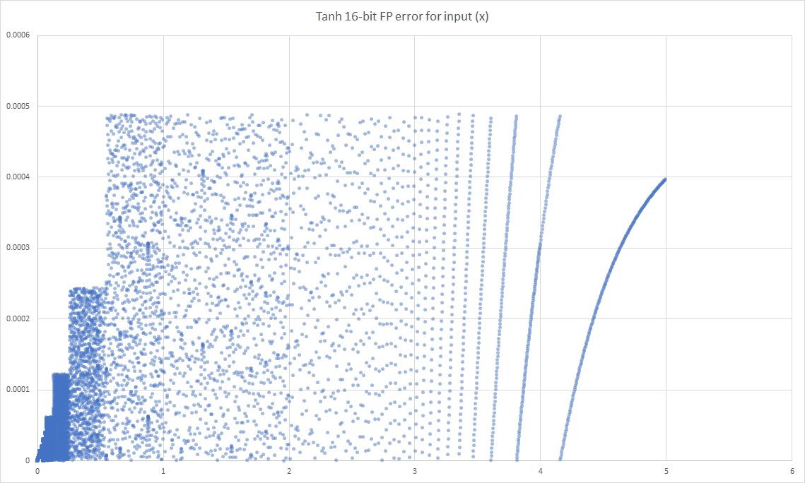
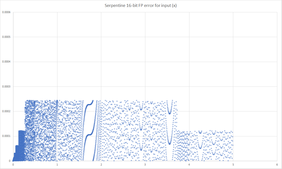
The error is calculated by taking every half-precision floating point value between 0.0 and 5 and passing it into the target function and measuring the different from the full 64-bit implementation, as opposed to the earlier work where we compared approximations to their source.

From this we can see that dropping to 16-bit floating point doesn’t incur any penalty to the functions with only linear component (Relu, LinearX, Constant) as these functions all take an input that exists in half-precision and return the same input or a fixed output that is also a valid half-precision number without any chance of overflow or rounding.

On the other hand our ‘tanh’ and ‘serpentine’ functions both perform calculations in half-float leading to errors which propagate to the return value. We can see by the median value that most results do no incur very much error at all but some values are very wrong.

Noticeably the approximation of the ‘Tanh’ function, ‘Serpentine’, has lower maximum and average error. To inspect this further we plotted the error for every input in the range 0.0 to 5.0 for both functions.

In both results the inherent pattern of the floating-point numbers is visible, but much noticeable on the ‘serpentine’ plot. The exact pattern is a little worrying as it changes the pattern from being close enough to ‘random’ to possibly having some implication in error propagation.

In our tests the network we used appears to be tolerant enough of either error and give good enough results for both - however the sigmoid-like ‘serpentine’ function is much cheaper than the ‘tanh’ which raises the question why it isn’t being used instead.

Additionally, the error across the range is non-linear for both. If we were to use this in a network the weights which allow for input closer to 0 will have a more diverse set of choices for values and allowing for a higher-precision fit than those with much larger activation values. This should result in a change in how the network converges on the correct answer.

More importantly is the propagation of error. In neural networks there is the problem of exploding and diminishing gradients which is commonly known (and one of the reasons for the popularity of non-linear but basically linear functions like ReLu). Allowing error to propogate through an application means that the combined error could cause unwanted behaviour such as that with gradients but also that the gradient you are using during back propagation may not be correct for the activation function that is being used.

This leaves us with the question of how tolerant are networks to small errors in the activation function, particularly with low precision data-types. Are there certain patterns of input or weights which in conjunction with non-linear error would slow or distort the learning process? Or will this type of error on larger networks limit the convergence onto the best possible solution?

Sometimes Activation Functions Only Vaguely Matter

This is a follow on from the last post where we discussed improving neural network performance by allowing for cheaper approximate functions to be used instead of the costly full-fat activation functions.

In Machine Learning an activation function is used to decide which neurons should be activated. It is a transform of the signal from layer to the next. To be able to fit to complex functions an activation layer must be non-linear otherwise the network is only capable of simple linear regression.

A list of common activation functions can be found on the wikipedia page which also gives the properties and limitations of each.

As you can see in that table, there is a lot and they seem to be very strictly defined. If we were to stick with ‘tanh’ as we looked at in the last post we could see it being implemented with more or less error. We were interested in figuring out if an implementation of ‘tanh’ which allowed an enormous amount of error, but was still non-linear, would be unable to perform the same task as the standard implementation of the ‘tanh’ function.

So we came up with two alternatives. ‘ApproxTanh3’ an order 3 polynomial approximation and ‘ApproxTanh12’ an order 12 polynomial approximation. The plot of these against the standard implementation can be seen below:

As you can see, the high order approximation is a reasonable fit to the actual tanh implementation where as the low order approximation basically falls off a cliff around x=0.5 .

So, what happens when we use this in a real neural network?

For this task we have chosen the standard MNIST handwriting dataset and a pretty simple convolutional neural network.

The dataset is a very common one, it is a collection of 28x28 pixel images of handwritten numbers and the number they represent. The standard test error rate of a convolutional neural network on this dataset is between ~0.2% and ~1.7% for different standard implementations.

And our neural network looks like this where {CHOSEN ACTIVATION} is either one of our approximations or the real ‘tanh’ implementation:

Conv2D(32, (5, 5), input_shape=(1, 28, 28), activation='relu')
MaxPooling2D(pool_size=(2, 2))
Dropout(0.2)
Flatten()
Dense(128, activation = {CHOSEN ACTIVATION} )
Dense(num_classes, activation='softmax')

With this network with the same seed we get these results:

Function	TEST ERROR RATE (%)
Keras.Tanh	0.97
ApproxTanh3	0.84
ApproxTanh12	1.31

This was very surprising to us. We expected the terrible order 3 approximation to break the ability for the neural network to fit the problem, but it’s results were within the ranges we expected and beat the standard implementations error rate in this specific seed (Other runs show some variance of +/- one percent).

In this example, our terrible activation function was able to match the standard implementation. It seems for certain problems where the inputs to the activation stay within certain ranges that the exact shape of the activation function isn’t important as long as it is vaguely correct within the working range.

This means that there is a large range of error tolerance in this system. A fact which it seems, for some networks, could be exploited to reduce learning times!

Improving the Performance of TensorFlow Activation Functions

In our research we are currently investigating existing applications which are tolerant to functions which return a value that is within a tolerance range rather than relying on absolute unit-in-last-place guarantees.

Machine-learning is a popular area of computing at the moment which just happens to conform to this paradigm. From specialised GPUs to TPUs we can see large teams approaching machine learning with variable precision stages and noise inducing layers to speed up or aid in the learning process.

While there is a lot of areas here which show levels of error tolerance, we have chosen to focus on the activation functions. In particular we are looking at the popular ‘tanh’ activation.

The function ‘tanh’ is a useful function due to its non-linearity and convenient output mapping of [-1,1]. Unfortunately, Tanh is an expensive function to compute accurately.

So, if we want to improve this we need to begin with the facts we know already:

• Some activation layers in a neural networks can be expensive

• Machine learning algorithms often use low-precision floats (16/32-bit)

• Floating-point cannot give absolutely correct answers for real numbers

• Inputs to some learning algorithms are often normalised to be values between zero and one

• Accuracy between zero and one in floating-point is non-linear. So error is higher in functions working closer to one

• Approximations of complex functions can result in better performance

• Machine learning is inherently error-tolerant

• Machine learning has a major problem with run-times being too long

From these facts we can assume:

1. The current ‘tanh’ function implementation has an acceptable and variable level of error

2. An approximation of ‘tanh’ which has better performance and acceptable levels of error will not impact on the overall outcome of the learning process and be valuable to the programmer

3. Any implementation which does not impact the overall result negatively and improves run-time would be a positive contribution.

So, if we want to show our assumptions apply to the real-world, we need to prove each one.

1) This is the simplest assumption to prove. The Tensorflow website provides a few machine learning tutorials, one of which is on Text Classification. This example uses a sigmoid activation in it’s final step. Changing this to a ‘tanh’ activation has no negative impact on the learning process. The accuracy of the output model remains in the 80-90% accuracy range.

Since we are using ‘tanh’ and the output is acceptable, the error that we know it has due to its underlying type must be valid and hasn’t impacted the convergence of the learning process.

2) Next we want to take an approximation and compare the result of using that to the official implementation to see if it has any difference characteristics which might be detrimental.

To do this we must select an implementation for the replacement. We have kept to a simple polynomial for this example as the resulting error is very small on the limited input range we are using ([0,1]). Although there are other, better performing, approximations with different costs associated.

With our replacement Activation function selected, we simple replace the final activation layer to point to our function and can then run the learning process. To ensure fairness between all implementations we use a fixed seed and reset the global state of Tensorflow for each run. This will allow us to see the ways in which the implementations may diverge through the learning process.

The tests give us the above results. The first chart is the standard implementation, while the other three are order-16 polynomials implementations in 64, 32 and 16-byte floating-point. As can be seen, there is very little difference between the approximations. The approximations do diverge from the official implementation around epochs 15-20. This divergence is expected due to the accumulation of small differences between the implementation but has no impact on the overall accuracy of the resulting model. In all tests that were ran the approximations and official implementation all converged to around the same accuracy.

This shows that the approximations do not negatively impact the overall result of the model.

NOTE: These tests were all trained on a CPU due to the NVIDIA libraries being non-deterministic. This non-determinism prevented 1-to-1 comparison of different activation functions with the same seed.

3) Next we need to consider the performance impact. As we are limited to working with a very small model due to problems with NVIDIA’s implementation preventing 1-to-1 testing on the GPU the activation layer is only a small part of a small model and this makes it difficult to accurately measure through the noise. To get around this we will be testing the implementations on the CPU separately (until we do further work with more time!).

Run on (8 X 3600 MHz CPU s)
CPU Caches: L1 Data 32K     (x4),  L1 Instruction 32K   (x4),
            L2 Unified 262K (x4),  L3 Unified 8388K     (x1)
------------------------------------------------------
Benchmark                                      Time  
------------------------------------------------------
Tanh Standard Implementation            |      212 ms 
                                        |
--Order 16 Polynomial Implementations-- |
SSE           64bit Float               |      114 ms 
Nonvectorised 64bit Float               |      144 ms 
SSE           32bit Float               |      114 ms 
Nonvectorised 32bit Float               |      129 ms 

Different machine learning libraries will take different approaches to vectorisation. As our functions are trivially vectorised on the CPU we see huge improvements over the standard ‘tanh’ performance, but we also see large improvements even in the standard scalar implementations.

A win of 25-50% on performance is significant when running a network with hours spent training, even if only a portion of that is spent with the activation functions.

Conclusion

With these three assumptions shown to be true in limited practice we are in a good position to make stronger assertions for larger neural networks and hopefully present a method to improve the performance of your Tensorflow models without having to make any tangible sacrifice!